You signed in with another tab or window. Reload to refresh your session.You signed out in another tab or window. Reload to refresh your session.You switched accounts on another tab or window. Reload to refresh your session.Dismiss alert
In the offline environment, session-level user-item interactions are mined to construct a weighted, bidirectional item graph.
The graph is then used to generate item sequences via random walks.
Item embeddings are then learned via representation learning (i.e., word2vec skip-gram), doing away with the need for labels.
Finally, with the item embeddings, they get the nearest neighbor for each item and store it in their item-to-item (i2) similarity map (i.e., a key-value store).
For Products on Homepage
In the online environment, when the user launches the app, the Taobao Personalization Platform (TPP) starts by fetching the latest items that the user interacted with (e.g., click, like, purchase).
These items are then used to retrieve candidates from the i2i similarity map.
The candidates are then passed to the Ranking Service Platform (RSP) for ranking via a deep neural network, before being displayed to the user.
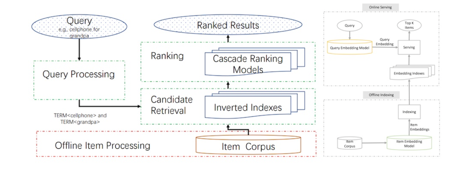
JD shared a similar approach for semantic retrieval for search
In the offline environment, a two-tower model with a query encoder and an item encoder is trained to output a similarity score for each query-item pair.
The item encoder then embeds catalog items before loading them into an embedding index (i.e., key-value store).
Then, in the online environment, each query goes through preprocessing (e.g., spelling correction, tokenization, expansion, and rewriting) before being embedding via the query encoder.
The query embedding is then used to retrieve candidates from the embedding index via nearest neighbors lookup.
The candidates are then ranked on factors such as relevance, predicted conversion, etc.
Tips to optimize model training and serving.
For model training, they raised that the de facto input of user-item interaction, item data, and user data is duplicative—item and user data appear once per row, consuming significant disk space.
To address this, they built a custom TensorFlow dataset where user and item data are first loaded into memory as lookup dictionaries.
Then, during training, these dictionaries are queried to append user and item attributes to the training set.
This simple practice reduced training data size by 90%.
Importance of ensuring offline training and online serving consistency.
For their system, the most critical step was text tokenization which happens thrice (data preprocessing, training, serving). - To minimize train-serve skew, they built a C++ tokenizer with a thin Python wrapper that was used for all tokenization tasks.
For model serving
They shared how they reduced latency by combining services.
Their model had two key steps: query embedding and ANN lookup.
The simple approach would be to have each as a separate service, but this would require two network calls and thus double network latency.
Thus, they unified the query embedding model and ANN lookup in a single instance, where the query embedding is passed to the ANN via memory instead of network.
They also shared how they run hundreds of models simultaneously, for different retrieval tasks and various A/B tests. Each “servable” consists of a query embedding model and an ANN lookup, requiring 10s of GB. Thus, each servable had their own instance, with a proxy module (or load balancer) to direct incoming requests to the right servable.
PS: The whole model is trained supervised with available ranking data.
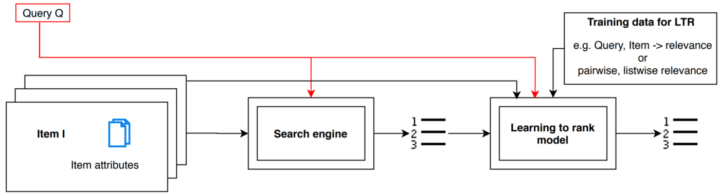
Traditional methods try to match a query with documents and derive relevance based on the similarity. Machine learning methods solve the IR problem by constructing a ranking model from a training data.
The system works by matching queries and documents and computing their similarity. Most similar documents are returned ranked by similarity with the query. Similarity is computed eg. as cosine similarity of TF-IDF vectors.
Learning to Rank systems often return an identical list of results to given query for all users, no personalization is involved.
Recommender systems do not use queries. They produce relevant items based on user history and similarities between users. Relevant items are computed by predicting their rating in the rating matrix or by recommending similar items based on their attributes.
Evaluating LTR and recommender systems:
CG
DCG
NDCG
Traditional learning to rank algorithms
Pointwise methods transform ranking into regression or classification of single items. The model then takes only one item at a time and either it predicts its relevance score or it classifies the item into one of the relevancy classes.
Pairwise methods tackle the problem as a classification of item pairs, i.e. deciding whether the pair of items belongs to the class of the pairs with the more relevant document at the first position or vice versa.
Listwise methods treat a whole item list as a learning sample. For example, by using all item scores belonging to one particular query and not by comparing pairs or single samples only.
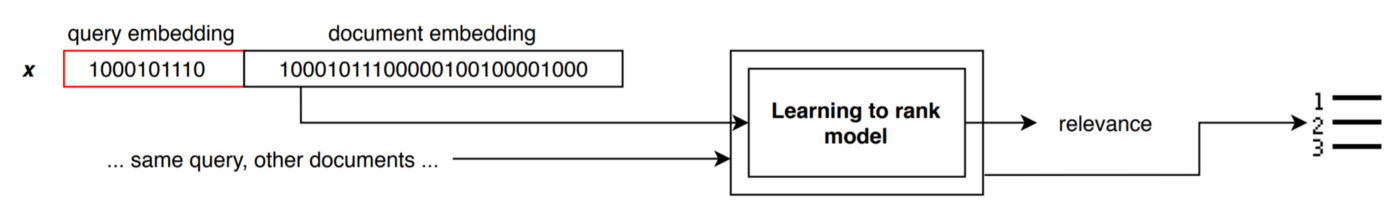
PRank algorithm uses Perceptron (linear function) to estimate the score of a document from a feature vector of this document. The query is appended to the feature vector of the document embedding. We can also classify documents into relevancy classes (e.g. relevant/irrelevant).
Rankboost directly optimizes the classification error. It is derived from Adaboost and works on document pairs. It trains weak classifiers giving more weight to pairs that were not correctly classified by ensemble in the previous step.
RankSVM was one of the first algorithms with pairwise approach to the problem. It approaches the ranking as ordinal regression, the thresholds of the classes have to be trained as well. RankSVM employs minimization of hinge loss function. It also allows direct use of kernels for non-linearity.
Motivation for listwise methods
Pairwise methods are very good, but they have drawbacks as well. Training process is costly and there is an inherent training bias that varies largely from query to query. Also only pairwise relationships are taken into account. We would like to use a criterion that allows us to optimize full list at simultaneously taking into account relevance of all items.
How to get training data for the LTR system?
Obtaining training data for the LTR system can be a lengthy and costly process. You typically need a cohort of human annotators entering queries and judging the search results. Relevance judgement is also difficult. Human assessors estimate one of the following scores:
Degree of relevance — Binary: relevant vs. irrelevant (good for pointwise)
Pairwise preference — Document A is more relevant than document B.
Total order — Documents are ranked as A,B,C,.. according to their relevance. (perfect for listwise, but exhaustive and time consuming)
It is apparent that human annotations are costly and their labels are not very reliable. One should therefore derive ranking and train the system from behavior of users on the website.
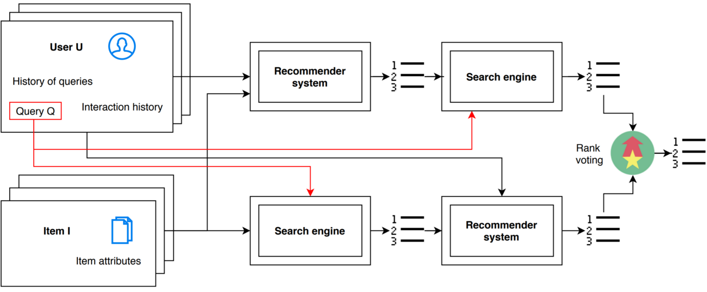
Even better approach is to replace the above described LTR algorithm with a recommender system.
Personalized search revisited
Knowledge based recommender systems
Both users and items have attributes. The more you know about your users and items, the better results can be expected.
For example, the item above is represented by several attributes that can be used to measure similarity of items. Then, recommendations are generated based on item similarity. When users are also described by similar attributes (e.g. text extracted from CVs of job applicants), you can recommend items based on user-item attributes similarities.
Note that in this case we do not use past user interactions at all. This approach is therefore very efficient for so called cold start users and items. Those are typically new users and new items.
Content based recommender systems
Such systems are recommending items similar to those a given user has liked in the past, regardless of the preferences of other users. Basically, there are two different types of feedback.
Explicit feedback is intentionally provided by users in form of clicking the “like”/”dislike” buttons, rating an item by number of stars, etc. In many cases, it is hard to obtain explicit feedback data, simply because the users are not willing to provide it. Instead of clicking “dislike” for an item which the user does not consider interesting, he/she will rather leave the web page or switch to another TV channel.
Implicit feedback data, such as “user viewed an item”, “user finished reading the article” or “user ordered a product”, however, are often much easier to collect and can also help us to compute good recommendations. Various types of implicit feedback may include:
Interactions (implicit feedback):
user viewed an item
user viewed item's details
user added an item to cart
user purchased an item
user have read an article up to the end
Again, you can expect better performance of recommender system, when the feedback is rich.
Content based recommenders work solely with the past interactions of a given user and do not take other users into consideration. The prevailing approach is to compute attribute similarity of recent items and recommend similar items. Recommending recent items themselves is often very successful strategy, which of course works just in certain domains and for certain positions.
Collaborative filtering
Last group of recommendation algorithms is based on past interactions of the whole user-base. These algorithms are far more accurate than the algorithms described in previous sections, when a “neighborhood” is well defined and the interactions data are clean.
KNN
Very simple and popular is a neighborhood-based algorithm (K-NN). To construct a recommendation for a user, k-nearest neighbor users (with most similar ranked items) are examined. Then, top N extra items (non-overlapping with items ranked by the user) are recommended.
This approach works perfectly fine not only for mainstream users and popular items, but also for “long-tail” users. By controlling how many neighbors are taken into the consideration for recommendation, one can optimize the algorithm and find a balance between recommending bestsellers and niche items. Good balance is crucial for performance of the system.
There are two major variants of neighborhood algorithms. The item-based and user-based collaborative filtering. Both algorithms operate on a matrix of user-item ratings.
Item-based v/s User-based
In the user-based approach, for user u, a score for an unrated item is produced by combining the ratings of users similar to u.
In the item-based approach a rating (u,i) is produced by looking at the set of items similar to i (interaction similarity), then the ratings by u of similar items are combined into a predicted rating.
The advantage of the item-based approach is that item similarity is more stable and can be efficiently pre-computed.
User-based algorithms outperform item-based algorithms in most of the scenarios and databases. The only exception can be databases with significantly lower number of items than users and low number of interactions.
Factorization based approaches
The matrix of interactions is factorized into two small matrices one for users and one for items with certain number of latent components (typically several hundreds). The (u,i) rating is obtained by multiplying of these two small matrices. There are several approaches how to decompose matrices and train them. The error can be minimized by Stochastic Gradient Descent, Alternating Least Squares or Coordinate Descent Algorithm. There are also SVD based approaches, where the ranking matrix is decomposed into three matrices.
