emp_pop_by_age.R

library(readabs)
library(tidyverse)
library(fpp3)
library(gganimate)

lfs_d_t1 <- read_abs("6291.0.55.001", "1")

emp_pop_age_sex <- lfs_d_t1 |> 
  filter(str_detect(series,
                    "Employment to population ratio"),
         !str_detect(series,
                     regex("Married",
                           ignore_case = TRUE)),
         str_sub(series, 1, 2) == ">>" |
           str_detect(series, "65 years and over")
  ) |> 
  separate_series(
    c("age", "indicator", "sex")
  ) |> 
  filter(sex != "Persons") |> 
  select(age, indicator, sex, date, value)

emp_pop_age_sex_withtot <- lfs_d_t1 |> 
  filter(series_id %in% c("A84591163L",
                          "A84592675K")) |> 
  separate_series(c("indicator", "sex")) |> 
  select(indicator, sex, date, value) |> 
  mutate(age = "Total (15+)") |> 
  bind_rows(emp_pop_age_sex)

seas_mod <- emp_pop_age_sex_withtot |> 
  mutate(date = yearmonth(date)) |> 
  as_tsibble(key = c(sex, age),
             index = date) |> 
  fill_gaps() |> 
  model(STL(value))

sa_emppop <- seas_mod |> 
  components() |> 
  select(sex, age, date, value = season_adjust) |> 
  mutate(date = as.Date(date))

# Plot! Emp-pop by age and sex over time ----

sa_emppop |> 
  ggplot(aes(x = date, y = value, col = sex)) +
  geom_line() +
  facet_wrap(~age) +
  theme_minimal() +
  scale_x_date(date_labels = "%b\n%Y",
                    breaks = seq(max(sa_emppop$date),
                                 min(sa_emppop$date),
                                 by = "-10 years")) +
  scale_y_continuous(labels = \(x) paste0(x, "%"),
                     limits = \(x) c(0, x[2]),
                     expand = expansion(c(0, 0.05))) +
  theme(legend.title = element_blank(),
        legend.position = "bottom",
        legend.direction = "horizontal",
        axis.title = element_blank(),
        panel.grid.minor = element_blank()) +
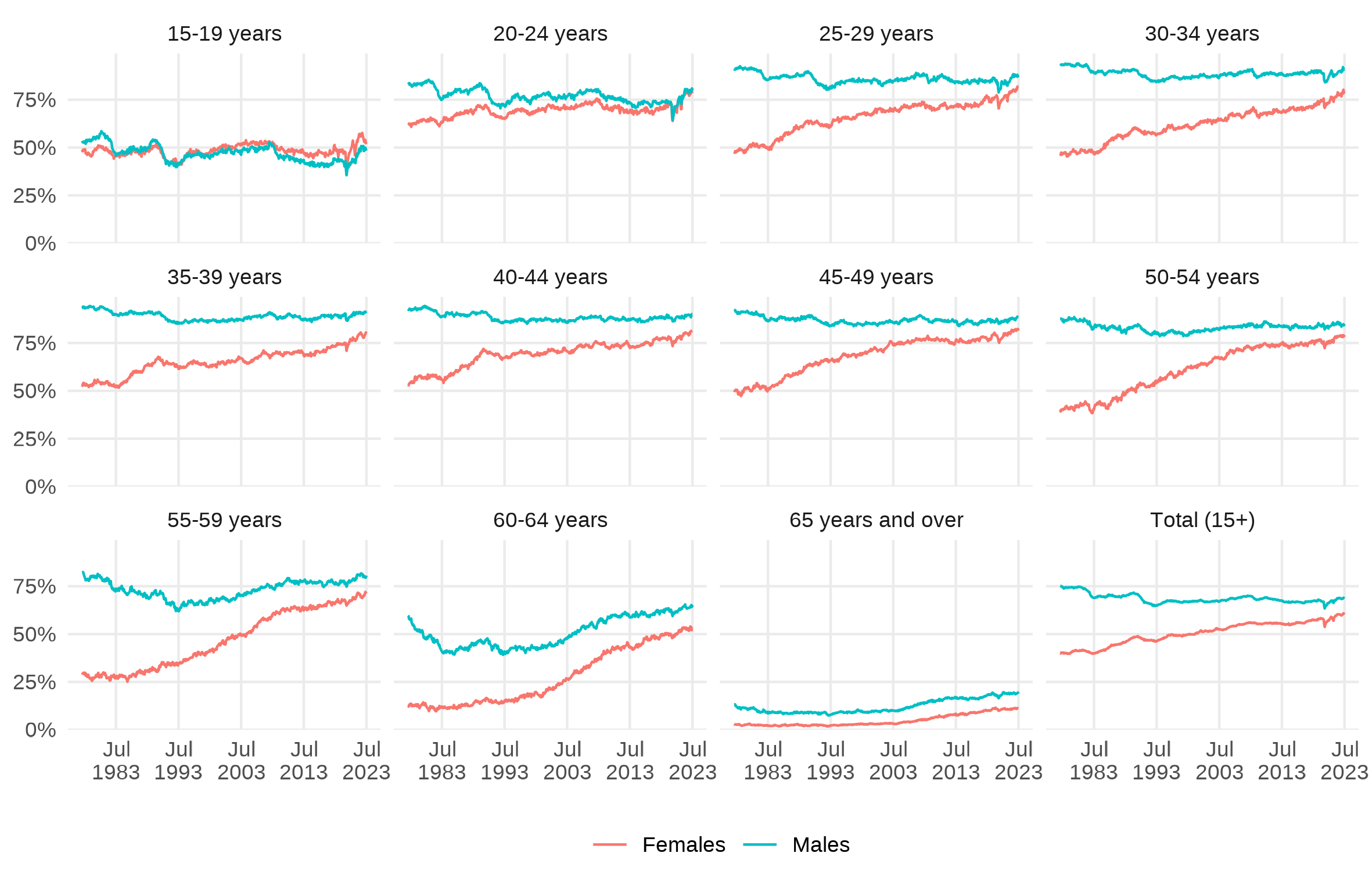
  labs(subtitle = "Employment to population ratio by age and sex, Australia",
       caption = "Source: ABS Labour Force Detailed. Seasonally adjusted using STL.")

# Make an animated plot! ----

anim_plot <- sa_emppop |> 
  filter(age != "Total (15+)") |> 
  mutate(age = str_remove_all(age, " years"),
         age = if_else(age == "65 and over", "65+", age),
         age_num = parse_number(str_sub(age, 1, 2)),
         pretty_date = format(date, "%b %Y")) |> 
  ggplot(aes(x = reorder(age, age_num),
             y = value,
             col = sex,
             group = sex)) +
  geom_line() +
  geom_point() +
  transition_time(date) +
  exit_fade(alpha = 0.05) +
  shadow_mark(alpha = 0.0175) +
  theme_minimal() +
  scale_y_continuous("", labels = \(x) paste0(x, "%")) +
  theme(legend.position = c(0.1, 0.1),
        legend.title = element_blank()) +
  labs(subtitle = "Australian employment-to-population ratio {format(frame_time, '%b %Y')}",
       x = "Age")

anim_save("emp_pop_by_age.gif",
          anim_plot,
          detail = 1,
          fps = 12,
          res = 220,
          width = 1500,
          height = 1000,
          units = "px",
          end_pause = 90,
          duration = 40,
          renderer = gifski_renderer())