Last active
February 8, 2025 10:54
-
-
Save MattCowgill/e81201ef8b2578c7e3f6bbb7c2ebe47b to your computer and use it in GitHub Desktop.
This file contains hidden or bidirectional Unicode text that may be interpreted or compiled differently than what appears below. To review, open the file in an editor that reveals hidden Unicode characters.
Learn more about bidirectional Unicode characters
| library(tidyverse) | |
| library(readrba) | |
| library(readabs) | |
| library(patchwork) | |
| theme_set(theme_minimal(base_size = 14) + | |
| theme( | |
| axis.title = element_blank(), | |
| axis.line.x = element_line(linewidth = 0.25), | |
| axis.ticks.x = element_line(linewidth = 0.25), | |
| panel.grid.minor = element_blank(), | |
| panel.grid.major.x = element_blank() | |
| )) | |
| inf_exp_raw <- read_rba_seriesid(c( | |
| "GUNIEXPY", | |
| "GUNIEXPYY", | |
| "GMAREXPY", | |
| "GMAREXPYY" | |
| )) | |
| inf_exp <- inf_exp_raw |> | |
| separate(series, | |
| c("source", "horizon"), | |
| sep = " – " | |
| ) |> | |
| mutate( | |
| source = str_remove_all(source, "' inflation expectations"), | |
| series = "Expected inflation" | |
| ) |> | |
| select(date, source, horizon, value) | |
| x_scale <- scale_x_date( | |
| limits = range(inf_exp$date), | |
| date_labels = "%Y", | |
| breaks = seq( | |
| max(inf_exp$date), | |
| min(inf_exp$date), | |
| "-10 years" | |
| ) | |
| ) | |
| plot_inf_exp <- inf_exp |> | |
| ggplot(aes(x = date, y = value, col = source)) + | |
| geom_line() + | |
| ggtext::geom_richtext( | |
| data = tibble( | |
| label = "<span style='color:#F8766D'>Market economists</span><br><span style='color:#00BFC4'>Union officials</span>", | |
| x = max(inf_exp$date), | |
| y = 6, | |
| horizon = "2-year ahead" | |
| ), | |
| aes_all(c("x", "y", "label")), | |
| inherit.aes = FALSE, | |
| hjust = 1, | |
| label.size = 0, | |
| size = 12 / .pt, | |
| vjust = 1 | |
| ) + | |
| facet_wrap(~horizon) + | |
| x_scale + | |
| labs(subtitle = "Expected inflation") + | |
| theme(legend.position = "none") | |
| plot_gap <- inf_exp |> | |
| pivot_wider( | |
| names_from = source, | |
| values_from = value | |
| ) |> | |
| mutate( | |
| value = `Union officials` - `Market economists`, | |
| series = "Difference in expected inflation" | |
| ) |> | |
| select(date, horizon, value, series) |> | |
| filter(!is.na(value)) |> | |
| ggplot(aes(x = date, y = value)) + | |
| geom_line() + | |
| facet_wrap(~horizon) + | |
| x_scale + | |
| labs(subtitle = "Difference in expected inflation") | |
| plot_inf_exp / | |
| plot_gap + | |
| plot_annotation(caption = "Source: RBA table G03.") |
Author
MattCowgill
commented
May 30, 2023

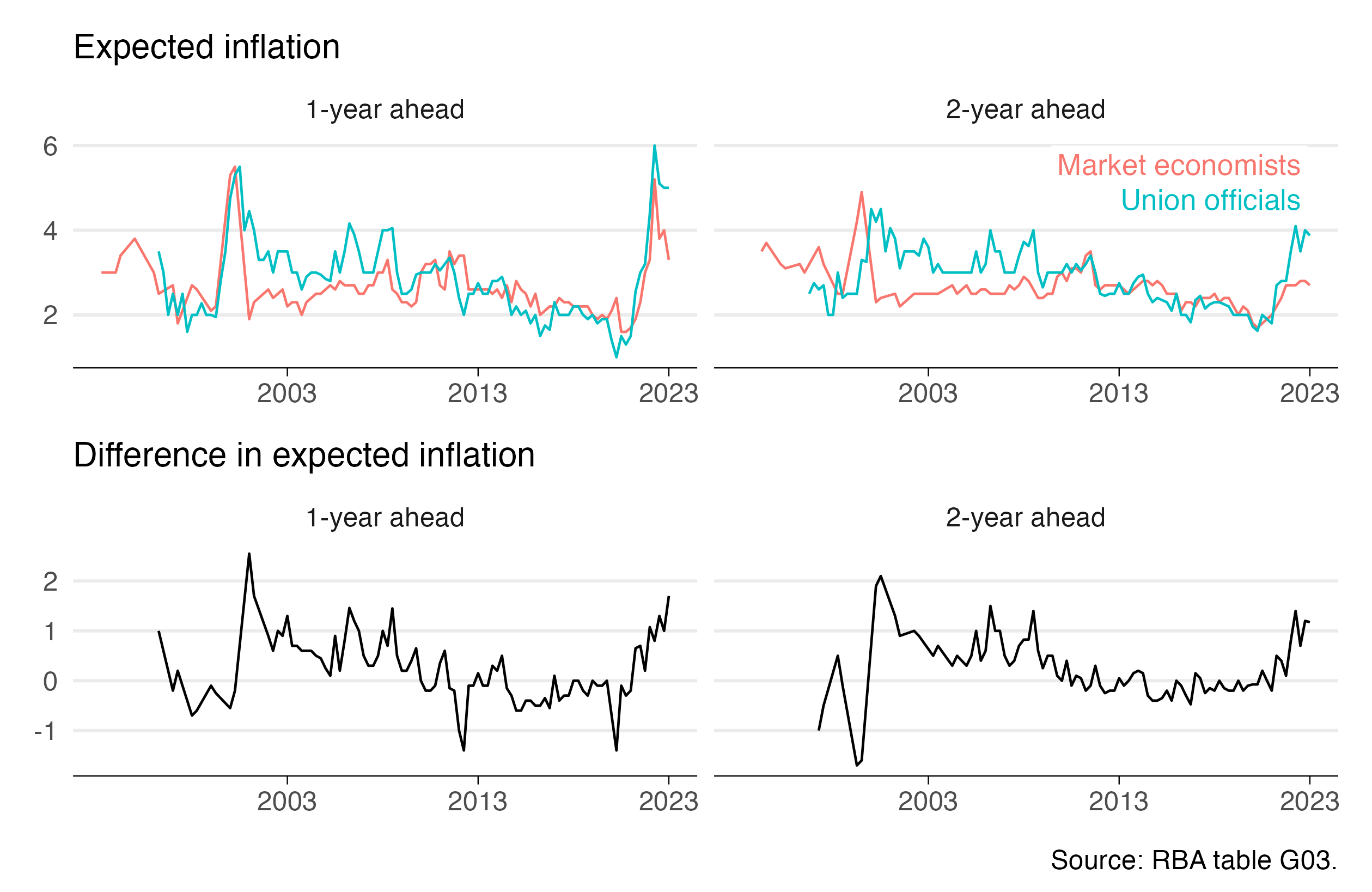
Curious if you compared this to actual inflation and which group tended to be more accurate e.g., using Brier score or something similar
@qwertytam I’ll leave that as an exercise for the reader!
Sign up for free
to join this conversation on GitHub.
Already have an account?
Sign in to comment