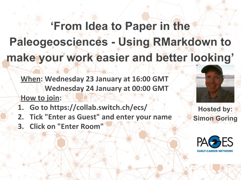
This webinar is set up as a "storytelling" session, about how I work through my projects that are intended for publication. In practice this is now how I manage most of my projects that involve some element of data exploration and collaboration. I will be live-coding during the presentation and intend to do so in a way that will allow people to follow along to some degree.
The webinar will be recorded and so people should not feel obligated to code along, or to keep up. If you would like to follow along, or revisit the webinar at a later date, these are the programs and R packages that you will need.
- Neotoma Slack channel link - https://bit.ly/2FrZyYD
- Presentation Sharing link - http://bit.ly/2MpqAAr
To follow along you must at minimum have:
We're going to make some files while we work, and also use some external files. In particular we'll be adding some bibliographic files. I generally work with plain text bib files, but you can use eml files with RMarkdown and pandoc. For this webinar I will use a BibTex file attached below as ecr_webinar.bib.
The first thing we do is download data from neotoma:
get_ds <- neotoma::get_dataset(gpid=c("Germany", "France", "Canada", "United States"))
We then wrap this in an if/else block to help us save time in the future when we render:
ds_file <- paste0("all_ds_v",version,".rds")
if(ds_file %in% list.files("data/output")) {
  get_ds <- readRDS(paste0("data/output/", ds_file))
} else {
  get_ds <- neotoma::get_dataset(gpid=c("Germany", "France", "Canada", "United States"))
  saveRDS(paste0("data/output/", ds_file))
}
We add a dynamic plot to the report:
neotoma::plot_leaflet(get_ds)We try to get the datasets without any site description elements using an lapply() function:
desc <- lapply(all_ds, function(x) {
    if (is.na(x$site.data$description)) {
      return(x)
    } else {
      return(NULL)
    }
  })

no_desc <- Filter(Negate(is.null), desc)