fit_to_activation.org

Fit to neuron activation plot

Relevant paper: https://journals.plos.org/plosone/article?id=10.1371/journal.pone.0218738

Confusion about the plots showing m_inf for SHL-1, see top left plot, red curve: https://journals.plos.org/plosone/article/file?type=supplementary&id=info:doi/10.1371/journal.pone.0218738.s003

Appendix with equations: https://journals.plos.org/plosone/article/file?type=supplementary&id=info:doi/10.1371/journal.pone.0218738.s001

Appendix with parameters used: https://journals.plos.org/plosone/article/file?type=supplementary&id=info:doi/10.1371/journal.pone.0218738.s002

According to this information the following equation is being used:

\begin{equation*}
m_{\text{SHL1,}\infty}(V) = \frac{1}{1 - \exp{\frac{-(V - V_h}{k_a}}} 
\end{equation*}

but in the paper this is referred to as a Boltzmann like distribution, e.g. p. 5 above equation (4).

This function however is essentially:

\begin{equation*}
f(x) = \frac{1}{1 - \exp{\frac{-x}}}
\end{equation*}

which has a singularity at $x = 0$, since $e^0 = 1$. See:

https://www.wolframalpha.com/input/?i=1+%2F+%281+-+e%5E%28-x%29%29

Which means it can’t be the function mentioned in the table / paper.

Boltzmann functions (not to be confused with Boltzmann distributions or the Maxwell-Boltzmann distribution) apparently are sigmoid like functions, see e.g.: https://www.graphpad.com/guides/prism/7/curve-fitting/reg_classic_boltzmann.htm

The function should thus be:

\begin{equation*}
m_{\text{SHL1,}\infty}(V) = \frac{1}{1 + \exp{\frac{-(V - V_h}{k_a}}} 
\end{equation*}

Note the + in the denominator instead of -.

Assuming this is a typo in the paper, let’s try to estimate whether the given parameters:

• $V_h = 11.2$
• $k_a = 14.1$

can match the plot mentioned above.

To do that we’ll extract some data points in a crude way from the plot above. Extract a cropped plot from the plot above, results in:

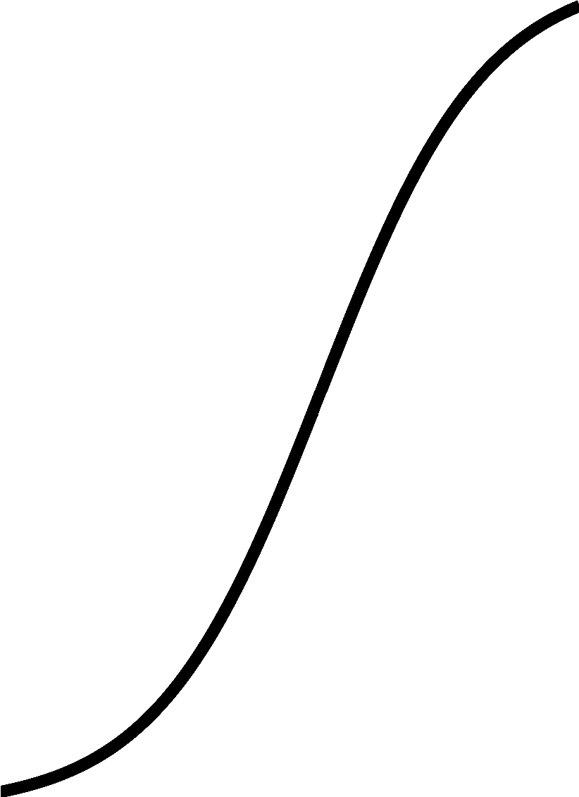
Now we write a small script to extract data points from this:

import flippy, os, sequtils, ggplotnim, cligen, strformat

proc toGrey(img: Image): seq[uint8] =
  case img.channels
  of 1: result = img.data
  else:
    result = newSeq[uint8](img.width * img.height)
    let nChannel = img.channels
    var val: int = 0
    var idx = 0
    for i in countup(0, img.data.high, nChannel):
      # calc mean of colors
      val = 0
      for j in 0 ..< nChannel:
        val += img.data[i + j].int
      result[idx] = 255 - (val div nChannel).uint8
      inc idx

proc allFalse(t: Tensor[bool]): bool =
  result = true
  for x in t:
    if x:
      return false

proc extractData(fname: string): seq[float] =
  let img = loadImage(fname)
  let rows = img.height
  let cols = img.width
  let imgTensor = toGrey(img).toTensor.reshape(rows, cols)
  let colIdx = arange(0, rows)
  result = newSeq[float](cols)
  var i = 0
  for idx, cl in enumerateAxis(imgTensor, 1):
    let sel = (cl >. 0).squeeze
    if not allFalse(sel):
      let idxs = colIdx[sel]
      let ind = mean(idxs)
      result[i] = (rows - ind).float / rows.float
    else:
      result[i] = 0.0
    inc i

proc scaleBy(s: var seq[float], low, high: float) =
  discard

proc main(fname: string,
          yLow = 0.0,
          yHigh = 1.0,
          xLow = 0.0,
          xHigh = 1.0) =
  var yVals = extractData(fname)
  yVals.scaleBy(yLow, yHigh)

  let xVals = linspace(xLow, xHigh, yVals.len)

  let df = seqsToDf(xVals, yVals)
  ggplot(df, aes("xVals", "yVals")) +
    geom_line() +
    ggsave("/tmp/extracted.pdf")

  df.write_csv(&"extracted_from_{fname.extractFilename}.csv")

when isMainModule:
  dispatch main

Finally, we can just perform a fit to those data points:

import math, ggplotnim, sequtils, strformat, mpfit

const ka = 14.1 # Parameter
const vh = 11.2

proc m_inf(V, vh, ka: float): float =
  result = 1.0 / (1 + exp( -(V - vh) / ka) )

proc buildDf(fn: proc(V, vh, ka: float): float): DataFrame =
  result = newDataFrame()
  let xt = linspace(-90.0, 90.0, 1000)
  result["xVals"] = xt
  result["yVals"] = xt.map_inline(fn(x, vh, ka))

proc fitToPaperPlot() =
  var df = toDf(readCsv("./extracted_from_m_inf_extract.png.csv"))

  # wrap the m_inf proc to fit
  let fnToFit = proc(p_ar: seq[float], x: float): float =
    result = m_inf(V = x, vh = p_ar[0], ka = p_ar[1])
  let xVals = df["xVals"].toTensor(float)
  let yVals = df["paperPlotY"].toTensor(float)
  let yErr = yVals.map_inline(1e-3) # guesstimate error...
  # fit to the data, start with paper parameters
  let (pRes, res) = fit(fnToFit,
                        @[11.2, 14.1],
                        xVals.toRawSeq,
                        yVals.toRawSeq,
                        yErr.toRawSeq)
  df["yFit"] = xVals.map_inline(fnToFit(pRes, x))
  df = df.gather(["paperPlotY", "yFit"], key = "Kind", value = "yVals")

  # add paper values
  var dfPaper = buildDf(m_inf)
  dfPaper["Kind"] = constantColumn("paperParams", dfPaper.len)
  echo dfPaper
  echo df
  df.add dfPaper

  echoResult(pRes, res = res)

  ggplot(df, aes("xVals", "yVals", color = "Kind")) +
    geom_line() +
    ylab("m_inf") +
    xlab("V / mV") +
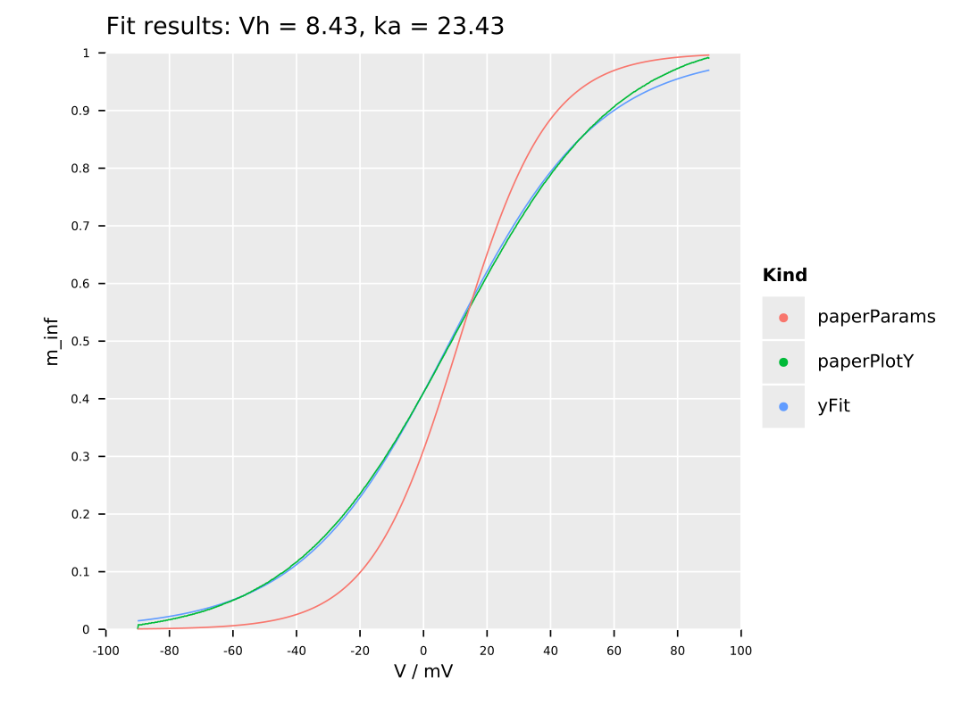
    ggtitle(&"Fit results: Vh = {pRes[0]:.2f}, ka = {pRes[1]:.2f}") +
    theme_opaque() +
    ggsave("/tmp/neuron_fit.png")

when isMainModule:
  fitToPaperPlot()

Which gives us the following final result: