Alexey Galakhov, 2024
We present an algorithm for interpolation S-curve jerk limited acceleration. Our algorithm can be implemeted as integer-only using ARM Cortex M4 vector instructions with only a few instructions per step, thus theoretically capable of generating 100s kHz of steps for multiple axes on a regular Cortex M4. The steps generated are always accurate, there is no error accumulation over time.
Most of stepper motor controller designs for 3d Printers and small CNC milling machines use STEP-DIR-based driving with steps generated in software. While cruise moves require just uniform step generation, acceleration and decceleration are much more complex due to their speed profiles.
The state-of-art acceleration (and decceleration) nowadays consider maximal velocity, acceleration and jerk (the first derivative of acceleration over time) in order to make movements as smooth as possible. Jerk-limited control is known to cause less vibrations and less acoustic noise compared to naive velocity-limited approach.
Note
The term jerk used here is not to be confused with the definition of "jerk" in Marlin firmware. Marlin defines >"jerk" just as sudden change of speed which has nothing to do with the S-Curve approach. We follow the usual definition of jerk used in classical mechanics.
In terms of change of speed over time, the jerk limited acceleration results in a so-called S-Curve speed profile. We discuss this in detail below.
Consider a movement of a single motor over time
is called velocity of the movement. The second derivative
is called acceleration. The third derivative
is called jerk. We don't need to consider further derivatives in our approach.
A movement has to be done with certain velocity. This may be less or equal to the maximal velocity
of the motor. Since we're not going to exceed this velocity, let's call it just maximal speed,
One can't just change motor velocity arbitrarely. The motor is only capable of deriving certain torque or force
The need of jerk limitation is less obvious. A real machanical system is not absolutely rigid. The transmission of the machine could be seen as a very strong spring and, in the first approach, described by the Hooke's law
giving us the maximal jerk,
The simplest approach taking into account only

If the jerk is limited, too, we get a more complex speed profile called S-curve for its shape.

There are seven segments on the speed profile:
- Ramp up the acceleration holding
$j = j_{max}$ until$a = a_{max}$ . - Hold
$a = a_{max}$ until velocity increases as needed. - Ramp down the acceleration holding
$j = -j_{max}$ until$a = 0$ . At this point$v = v{max}$ is reached. - Hold
$v = v_{max}$ until coordinate changes as needed. - Ramp up the decceleration holding
$j = -j_{max}$ until$a = -a_{max}$ . - Hold
$a = -a_{max}$ . - Ramp down the decceleration holding
$j = j_{max}$ until$a = 0$ , reaching$v = 0$ and$x$ reaching the target position.
In shorter movements the
We could investigate a more general case. Consider the machine changing from velocity

For the purpose of interpolation we need the coordinate, not the velocity. The corresponding coordinate graph is shown at the Figure.

The generalized goal can be now written as follows: consider the machine being at
Note that every segnment of the movement is essentially a cubic polynomial. In its most general form it could be written as
which is also true for cruise movement (
There is another form of the polynomial in question without explicit usage of
One remarkable special case of cubic polynomials are cubic Bézier curves. They are especially interesting for realtime tasks due to existance of the de Casteljau's algorithm. This algorithm finds arbitrary point on given Bézier curve using only few multiplications and additions and can be implemented using solely fixed-point arithmetics, that is, integers. It is a perfect fit for SIMD instructions found on Cortex M4 and bigger processors.
Fortunately there is direct correspondence between Bézier curves and acceleration S-curve. Each acceleration step corresponds to a Bézier segment. The control points have to be placed as shown on the figure below:

The time of each segment (denoted
Both velocities are then used to place control points. In fact, both control points are these velocities represented as some coordinates. The 2nd control point is the coordinate we would reach if we would move with
Generally, Bézier curves are described in parametric form and there is no simple way to integrate along them in coordinate form. However in our special case there is a simple relation between the parameter and the time. Choosing control points at
This could easily be proven by substituting this for
Now we got the recipe for converting the polynomial into control points of a Bézier curve:
Let's define waypoint as a point in the configuration space
In order to move from waypoint
Now, taking the parameter
The de Casteljau's algorithm of Bézier interpolation can be implemented as a series of linear interpolations. There is a beautiful animation of what we're going to do (source: Wikipedia):
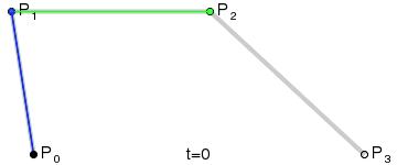
On this image
The computation is as follows:
Note that the algorithm is nothing else than six repeats of the same operation, linear interpolation between two points. In the program code we would get something like
fn interp(p: Number, a: Number, b: Number) -> Number {
    p * b + (1 - p) * a
}

let q0 = interp(p, p0, p1);
let q1 = interp(p, p1, p2);
let q2 = interp(p, p2, p3);
let r0 = interp(p, q0, q1);
let r1 = interp(p, q1, q2);
let x = interp(p, r0, r1);
Let's analyze numerical stability of the above code. The critical part is, we must land at p = 1. In this case (1 - p) == 0 and interp(1, a, b) == b respectively, since both multiplication and addition do not lose precision in case of working with just 0 and 1. As a result, we get x == p3.
The smoothness of the transition between segments is guaranteed by the properties of Bézier curves. Note that we use explicit velocities at waypoints. Our algorithm guarantees that the waypoint will be reached precisely including its velocity, even if there is some deviation in the middle of the segment. Note that the algorithm is symmetrical in respect to segment ends, and there is no difference between the starting endpoint and the ending one. We could swap them by swapping
In real world a trajectory interpolator must something change its mind. Consider we're in the middle of some segment and we get some new command from either the user or the machine endstop. We must abandon our current movement and continue with the new one.
Fortunately, Bézier curves provide the necessary functionality without any algorithm changes. The only thing we need to do is to track the current velocity. We don't even need to compute it separately since it is already present in our algorithm in the form of
The algorithm itself does not limit neither
Another consideration is, there may be global change of the machine feedrate. In this case we should move faster or slower - globally. In order to do so, we don't need to recompute velocities. As soon as all machine axes have the same override, the only thing we need to do is to change the interpolation parameter. That is, just let run the time slower or faster. This is achieved by
where
The structure of the interp() function allows for easy using of fixed-point numbers. For example, let's use 16-bit arithmetics. For efficiency let's represent 1 as 1 << 16. This would mean that we can't use 1 directly, but since we only reach
Doing so, we multiply by p with the following bit-shift 16 bits to the right. Such a bit-shift is "free of charge" on many of current CPU architectures. Similarly, the 1-p becomes just the overflowing subtraction from zero, that is, negating. In fixed-point numbers our interpolation function gets the following form:
fn interp(p: u16, a: i32, b: i32) -> i32 {
    (b * (p as i32) >> 16) + (a * (0.overflowing_sub(p).0 as i32) >> 16)
}
While arithmetic right shift is not exactly the same as division, this introduces less than one bit error and can be neglected provided that i32 denotes microsteps or sub-microsteps. Here we assume that the multiplication does not overflow. If the precision is higher, one should use 64-bit numbers instead.
Note that all multiplications in all calls of interp() use the same p and 0.overflowing_sub(p). This allows for these values to be calculated in advance and stored in a register. After that, vector instructions can be used to do multiple multiplications at once. Here is an example of machine code for the complete Bézier interpolation in one dimension for a Cortex M4, as generated by rustc 1.79.0:
push	{r4, r5, r6, r7, r8, lr}
smull	ip, lr, r1, r0
rsb	r1, r0, #65536	@ 0x10000
smull	r4, r5, r2, r0
smlal	ip, lr, r1, r2
ldr	r2, [sp, #24]
smull	r8, r7, r3, r0
smlal	r4, r5, r1, r3
smlal	r8, r7, r1, r2
lsl	r2, lr, #16
orr	r2, r2, ip, lsr #16
lsl	r5, r5, #16
smull	r2, r3, r2, r0
orr	r5, r5, r4, lsr #16
lsl	r7, r7, #16
smull	r4, r6, r5, r0
orr	r7, r7, r8, lsr #16
smlal	r2, r3, r5, r1
smlal	r4, r6, r7, r1
lsl	r3, r3, #16
orr	r2, r3, r2, lsr #16
smull	r0, r2, r2, r0
lsl	r3, r6, #16
orr	r3, r3, r4, lsr #16
smlal	r0, r2, r3, r1
lsr	r0, r0, #16
orr	r0, r0, r2, lsl #16
pop	{r4, r5, r6, r7, r8, pc}
As we can see, the compiler is able to generate very efficiend code using smull and smlal instructions. Alternative code generated with some manual hints uses smuad instruction. The computation part of it looks like this:
pkhbt	r0, r1, r0, lsl #16
sub	r4, r4, ip
pkhbt	r1, r3, r2, lsl #16
pkhbt	r4, r4, ip, lsl #16
smuad	ip, r4, lr
lsr	r2, ip, #15
smuad	r0, r4, r0
lsl	r0, r0, #1
smuad	r1, r4, r1
pkhtb	r0, r0, ip, asr #15
lsr	r1, r1, #15
smuad	r0, r4, r0
pkhbt	r1, r1, r2, lsl #16
smuad	r1, r4, r1
lsr	r1, r1, #15
pkhbt	r0, r1, r0, lsl #1
smuad	r0, r4, r0
lsr	r0, r0, #15
This requires however much more preparations and is only efficient if interpolating multile axes at once.
The computation is small enough to be placed directly in a timer interrupt. The suggested architecture is as follows:
- A list of waypoints is maintained. There is always exactly one next active waypoint.
- The timer interrupt interpolates towards the next active waypoint all the time.
- As soon as the next active waypoint is reached, the timer interrupt takes the next one from the list.
- The planner feeds waypoints into the list. It also can change the next active waypoint on the fly, which corresponds to re-planning.
- The list must be always fed unless the velocity is zero. It is an emergency if the waypoint list gets empty at non-zero velocity ("we're moving but we don't know where to move").
- The algorithm of step generation is always the same regardless of the complexity of the move. One only needs to provide correct waypoints.
- All usual Bézier curve properties apply, including the one that the whole segment lies inside the polygon of its control points. No overshoots are possible.
- Waypoints only require coordinates and velocities. They can be calculated anywhere by any means and fed in any way, including USB connections.
- The interpolator doesn't have any parameters like maximal acceleration or jerk. It takes them from waypoints.
- The waypoint is always reached with maximal precision possible. Errors do not accumulate over time and reach their maximal values in the middle between two waypoints. Coordinate error at any waypoint is always exactly zero.
- The algorithm is much less efficient on processors lacking DSP or SIMD instructions. It is not suitable for 8-bit MCUs in its present form.
- There is no advantage in constant-velocity moves. The computation is always the same.
- Waypoint calculation is always to be done in advance. Failure to feed waypoints results in an immediate emergency stop.
- It is only possible to generate steps on time-driven basis. It is impossible to calculate the time until the next step.
- We generate coordinates, not steps. The coordinate must be compared to the previous one in order to determine
STEPandDIRunless we use a servo motor taking absolute coordinate at its input. - Nothing but careful planning guarantees that there will be no two steps at once or that the velocity and acceleration are not too high.
- We need to know time between waypoints in advance. This is the price we must pay for not having explicit acceleration and jerk parameters.
- Figures like circles must be approximated with polynomial pieces. This however doesn't really lose the precision since even with few segments the chord error of less than one microstep can be achieved.
- Using Bézier curves as the trajectory planner input has no advantages since we can't interpolate an arbitrary Bézier curve. The algorithm only works for a very special subset of them. The general case is known to be analytically insolvable.