-
- What is TensorFlow?
- 1.1. Introduction
- 1.2. Design principles
- 2.0 TF Execution model
- 2.1. Dataflow graph elements
- 2.2. Partial and concurrent execution
- 2.3. Distributed execution
- 2.4 Dynamic control flow
- 2.5 Differentiation and optimization
- 3.0 Building a model
- 3.1 Modeling a Neural Network
- Loose Concepts
- Libraries and Extensions
- Why do you need virtual environments to run TF?
- Session and InteractiveSession
- Don't start from scratch
- TensorFlow vs. the competition
- 1.1. Introduction
- What is TensorFlow?
-
- What is Keras?
-
- TensorFlow 2.0 What changes?
- 3.1 Main Changes
- 3.2 Recommendations for idiomatic TF 2.0
- 3.3 Depolying
- 3.4 Coverting to TF-Lite
- 3.5 Run inference with the model
- 3.6 Optimize you model
- TensorFlow 2.0 What changes?
TensorFlow is open-source!
TensorFlow is an open source library for numerical computation and large-scale machine learning. TensorFlow bundles together a slew of machine learning and deep learning (aka neural networking) models and algorithms and makes them useful by way of a common metaphor. It uses Python to provide a convenient front-end API for building applications with the framework, while executing those applications in high-performance C++. With TF is possible to train and run neural networks for handwritten digit classification, image recognition, word embeddings, recurent neural networks, sequence-to-sequence models for machine translantion, natural languange processing, and PDE (partial differential equation) based simulations. TF supports production prediction at scale, with the same models used for training.
TF has been evolved since first-generation system. It supports both large-scale training and inference: it efficiently uses hundreds of powerful (GPU-enable) servers for fast training, and it runs trained models for inference in production on various platforms, ranging from large distributed clusters in a datacenter, down to running locally on mobile devices. At same time, it is flexible enough to support experimentation and research into new machine learning models and system-level optimizations.
TensorFlow uses a unified dataflow graph to represent both the computation in an algorithm and the state on which the algorithm operates. Unlike traditional dataflow systems, in which graph vertices represent functional computation on immutable data, TensorFlow allows vertices to represent computations that own or update mutable state. Edges carry tensors (multi-dimensional arrays) between nodes, and TensorFlow transparently inserts the appropriate communication between distributed subcomputations.
By unifying the computation and state management in a single programming model, TensorFlow allows programmers to experiment with different parallelization schemes that, for example, offload computation onto the servers that hold the shared state to reduce the amount of network traffic. Also have various coordination protocols, with encouraging results with synchronous replication, echoing recent results that contradict the held belief that asynchronous replication is required for scalable learning.
TF provides a simple dataflow-based programming abstraction that allows users to deploy applications on distributed clusters, local workstations, mobile devices, and custom-designed accelatores. A high-level scripting interface (Fig.1) wraps the construction of dataflow graphs and enables users to experiment different model architectures and optimization algorithms without modifying the core system.
Dataflow graphs of primitive operators TF use a dataflow representation for their models, and ith can represent individual mathematical operators (such as matrix multiplication, convolution, ect) as nodes in the dataflow graph. This makes it easier for users to compose novel layers using high-level scripting interface. Many optimization algorithms require each layer to have defined gradients, and building layers out of simple operators make it easy to differentiate these models automatically. In addition to the funcional operators, is represented a mutable state, and the operations that pdate ir, as nodes in the dataflow graph, thus enabling experimentation with different update rules.
Deferred execution A typical TF apllication has two distinct phases: the 1º defines the program (e.g. neural network to be trained and the update rules) as a symbolic dataflow graph with placeholders for the input data and variables that represent the state; and the 2º phase executes an optimized version of the program on the set of avaible devices. By deferring the execution until the entire program is available, TF can optmize the execution phase by using global information about the computation. E.G. TF achives high GPU utilization by using the graph's dependency structure to issue a sequence of kernels to the GPU without waiting for intermediate results. This design makes exection more efficient, however is needed to push more complex features - such as dynamic control flow - into the dataflow graph, so that models using these features enjoy the optimizations.

Fig.1 A schematic TensorFlow dataflow graph for a training pipeline, containing subgraphs for reading input data, preprocessing, training, and checkpointing state.
TF is based on the concept of the data flow graph. The nodes of this graph represent operations, the edges are tensors (explained below).
TF uses a single dataflow graph to represent all computation and state in a machine learning algorithm, including the individual mathematical operations, the parameters and their update rules, and the input pre-processing.
The key observation in the parameter server architecture is that mutable state is crucial when training very large models, because it is possible to make in-place updates to very large parameters, and propagate those updates to parallel training steps as quickly as possible. DataFlow with mutable state enables TF to mimic the functionality of a parameter server, but with additional flexibility, because it becomes possible to execute arbirtrary dataflow subgraphs on the machines that host the shared model parameters.
In a tensorflow graph, each vertex represents a unit of local computation, and each edge represents the output from, or input to, a vertex. Refer to the computation at vertices as operations, and the values that flow along edges as tensors.
Tensors TF model all data as tensors (n-dimensional arrays) defined by the properties Rank, Shape, and Type. Fig.19

Fig.19 - Description of Tensors Rank
Constants, Variables and Placeholders are the possible types of a Tensor. They represent the inputs to and results of the common mathematical operations in many machine learning algorithms.
* __Placeholders__ are values that are unassigned and will be initialized by the session when run, and always need to be fed when running the session. __Variables__ are values that can change and __Constants__ are values that don't change.
After create the Tensor is possible to acess and change some specifications with methods like get_shape()and reshape().
Graph TensorFlow computations can be represented as data flow graphs. Each graph is built as a set of Operation objects.
Operations An operations takes m >= 0 tensors as input and produces n >= 0 tensores as output. An operations has a named 'type' (such as Const, Matmul or Assign) and may have zero or more compile-time attributes that determine its behaviour. An op can be polymorphic and variadic at compile-time: its attributes determine both the expected types and arity of its inputs and outputs.
Session This is an entity that represents an environment for running calculations on the data flow graph.
E.G.
#Operations with matrices as graph input flow
	a = tf.placeholder(tf.types.float32, shape=(2, 4))
	b = tf.placeholder(tf.types.float32, shape=(4, 2))

	# Apply multiplication
	mul = tf.matmul(a, b)

	# Construct a `Session` to execute the graph
	sess = tf.Session()

	# Import Numpy
	import numpy as np

	# Create matrices with defined dimensions and fill them with random values
	rand_array_a = np.random.rand(2, 4)
	rand_array_b = np.random.rand(4, 2)

	# Execute the graph and print the resulting matrix
	print sess.run(mul, feed_dict={a: rand_array_a, b: rand_array_b})

	# Close the session
	sess.close()

    #Output
    [[ 1.32082355  0.97404259]
    [ 1.06961715  1.15667367]]
The API for executing a graph allows the client to specify declaratively the subgraph that should be executed. The client selects zero or more edges to feed input tensors into the dataflow, and one or more edges to fetch output tensors from the dataflow; the runtime then prunes (podar - (de podar árvores)) the graph to contain the necessary set of operations. Each invocation of the API is called a step, and TensorFlow supports multiple concurrent steps on the same graph.
Stateful operations allow steps to share data and synchronize when necessary. Fig.1 shows a typical training application, with multiple subgraphs that execute concurrently and interact through shared variables and queues. The core training subgraph depends on model parameters and input batches from a queue. Many concurrent steps of the training subgraph, update the model based on different input batches, to implement data-parallel training. To fill the input queue, concurrent preprocessing steps transform individual input records (e.g., decoding images and applying random distortions), and a separate I/O subgraph reads records from a distributed file system.
TF flexibility is mostly associated with partial an concurrent execution.
By default, concurrent executions of a TensorFlow subgraph run asynchronously with respect to one another. This asynchrony makes it straightforward(simples/evidente) to implement machine learning algorithms with weak consistency requirements, which include many neural network training algorithms.
Dataflow simplifies distributed execution, because it makes communication between subcomputations explicit. It enables the same TensorFlow program to be deployed to a cluster of GPUs for training, a cluster of TPUs for serving, and a cellphone for mobile inference.
Each operation resides on a particular device, such as a CPU or GPU in a particular task. A device is responsible for executing a kernel for each operation assigned to it. TensorFlow allows multiple kernels to be registered for a single operation, with specialized implementations for a particular device or data type. For many operations, such as element-wise operators (Add, Sub, etc.), we can compile a single kernel implementation for CPU and GPU using different compilers.
The placement algorithm computes a feasible set of devices for each operation, calculates the sets of operations that must be colocated, and selects a satisfying device for each colocation group. It respects implicit colocation constraints that arise because each stateful operation and its state must be placed on the same device. In addition, the user may specify partial device preferences such as “any device in a particular task”, or “a GPU in any task”, and the runtime will respect these constraints. A typical training application will use client-side programming constructs to add constraints such that, for example, parameters are distributed among a set of “PS” tasks. Fig2.

Fig.2 - This diagram illustrates TF general architecture.
In conclusion, TF allows great flexibility in how operations in the dataflow graph are mapped to devices.
TF was optimized for executing large subgraphs repeatedly with low latency. Once the graph for a step has been pruned, placed, and partitioned, its subgraphs are cached in their respective devices. A client session maintains the mapping from step definitions to cached subgraphs, so that a distributed step on a large graph can be initiated with one small message to each participating task. This model favors static, reusable graphs, but it can support dynamic computations using dynamic control flow.
TF supports advanced machine learning algorithms that contain conditional and interative control flow. E.G. a recurrent neural network (RNN) such as LSTM can generate predictions from sequential data. Google's Neural Machine Translation system uses TF to train a deep LSTM that achives state_of_the_art performance on many translations tasks. The core of an RNN is a recurrence relation, where the output for sequence element i is a function of some state that acumulates across the sequence. In this case, dynamic crontrol flow enables iteration over sequences that have variable lengths, without unrolling the computation to the length of the longest sequence.
As seen, TF uses deferred execution via the dataflow graph to offload larger chunks of work to accelerators. Therefore, to implement RNNs and other advanced algorithms, we add conditional (if statement) and iterative (while loop) programming constructs in the dataflow graph itself. We use these primitives to build higher-order constructs, such as map(), fold(), and scan().
For this purpose, we borrow the Switch and Merge primitives from classic dynamic dataflow architectures.
Switch operation forwards data to the output port determined by pred. If pred is true, the data input is forwarded to output_true. Otherwise, the data goes to output_false. Switch receives two inputs. One of them is a predicate, which is boolean tensor (true or false), and another one is the data that should be passed. Predicate determines whether the data should be passed by output_true branch or output_false branch. But, one weird stuff here is the concept of the dead tensor. No matter whether the predicate is true or false; always there are two outputs: one of them is data and the other one is the dead tensor. If pred is true, the dead tensor is sent along output_false(and vice versa).
First of all, dead tensors are an implementation detail of TensorFlow’s control flow constructs:
tf.cond()andtf.while_loop(). These constructs enable TensorFlow to determine whether or not to execute a subgraph based on a data-dependent value. E.G., When a tensor receives a dead tensor as one of its input, it doesn't execute; instead it sends a dead tensor on all of its outputs. This dead-tensor propagation ensures that only the ops in the appropriate branch will execute.
Merge can receive more than one inputs, but only one of them must contain the data and others should be the dead tensors. Otherwise, we will face with some random and unpredictable behavior. The conditional operator uses Switch to execute one of two branches based on the runtime value of a boolean tensor, and Merge to combine the outputs of the branches. The while loop is more complicated, and uses Enter, Exit, and NextIteration operators to ensure that the loop is well-formed.
https://towardsdatascience.com/tensorflow-control-flow-tf-cond-903e020e722a
Optimizers are extended class, which includes added information to train a specific model. The optimizer class is initialized with given parameters and are used to improve speed and performance for training a specific model and are often method for minimizing loss. The basic optimizer of TF is tf.train.Optimizer. Some od TF optimizers are : Stochastic Gradient descent , Stochastic Gradient descent with gradient clipping, Momentum, Nesterov momentum, Adagrad, Adadelta, RMSProp, Adam, Adamax, SMORMS3.
https://www.tensorflow.org/api_docs/python/tf/keras/optimizers
The mechanism beahind optimizers operations are mathematical and you can find more information about them @here.
https://en.wikipedia.org/wiki/Stochastic_gradient_descent
TF users can also experiment with a wide range of optimization algorithms, which compute new values for the parameters in each training step, like biases, a bias value allows you to shift the activation funtion to the left or right, which may be critical for successful learning. It might help to look at a simple example. Consider this 1-input, 1-output network that has no bias: Fig.4

Fig.4 - Scheme of 1 input, 1 output network that has bo bias.
The output of the network is computed by multiplying the input (x) by the weight (w0) and passing the result through some kind of activation function (e.g. a sigmoid function.) Here is the function that this network computes, for various values of w0:Fig.5

Fig.5 - Function that this network computes, for various values of w0.
Changing the weight w0 essentially changes the "steepness" of the sigmoid. That's useful, but what if you wanted the network to output 0 when x is 2? Just changing the steepness of the sigmoid won't really work -- you want to be able to shift the entire curve to the right. That's exactly what the bias allows you to do. If we add a bias to that network, like so: Fig.6 then the output of the network becomes sig(wox +w11.0).This is what the output look like for various values of w1: Fig.7 Having a weight of -5 for w1 shifts the curve to the right, which allows us to have a network that outputs 0 when x is 2.

Fig. 6 - Same scheme when added bias, then the output of the network becomes sig(w0x + w11.0).

Fig.7 - Function representing output of the network for various values of w1.
https://stackoverflow.com/questions/2480650/role-of-bias-in-neural-networks
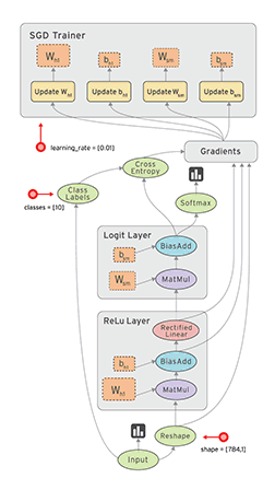
A neural network is build layer by layer. First, you must define placeholders for inputs and labels because you normally won't put in the 'real' data yet. Then the first start is model the input data according to whether you need, usually an 'operation' correspond to a layer. The way you construct your layers define de neural network Architectures. Fig.20

Fig.20 - Simple representation of general neuron architecture.
The top 10 most implemented Neural Networks
1 - Perceptrons (MLP) Considered the first generation of neural networks, Perceptrons are simply computation models of a single neuron. Also called feed-forward neural network, perceptron feeds informations from the front to the back. Training perceptrons usually requires back-propagations, giving the network paired datasets of inputs ans outputs. Inputs are sent into the neuron, processed, and result in an output. The error being back propagated is often some variation of the difference between the input and the output. Given that the network has enough hidden neurons, it can theoretically always model the relationship between the input and output. Practically their use is a lot more limited but they are popularly combined with other networks to form new networks. Fig.8

Fig.8 - Illustrated relationship between the input and output of MLP.
2- Convolutional Neural Networks (CNN) These are primarily used for image processing but can also be used for other types of input such as audio. A typical use case for CNN is where you feed the network images and the network classifies the data. CNNs tend to start with an input “scanner” which is not intended to parse all the training data at once. For example, to input an image of 100 x 100 pixels, you wouldn’t want a layer with 10 000 nodes. Rather, you create a scanning input layer of say 10 x 10 which you feed the first 10 x 10 pixels of the image. Once you passed that input, you feed it the next 10 x 10 pixels by moving the scanner one pixel to the right. Fig.9 e Fig.10

Fig.9 - Architecture of CNN

Fig.10 - Representative architecture of CNN of concrete example.
This input data is then fed through convolutional layers instead of normal layers, where not all nodes are connected to all nodes. Each node only concerns itself with close neighboring cells. These convolutional layers also tend to shrink as they become deeper, mostly by easily divisible factors of the input. Besides these convolutional layers, they also often feature pooling layers. Pooling is a way to filter out details: a commonly found pooling technique is max pooling, where we take say 2 x 2 pixels and pass on the pixel with the most amount of red.
3- Recurrent Neural Networks(RNN) When applying machine learning to sequences, we often want to turn an input sequence into an output sequence that lives in a different domain; for example, turn a sequence of sound pressures into a sequence of word identities. When there is no separate target sequence, we can get a teaching signal by trying to predict the next term in the input sequence. The target output sequence is the input sequence with an advance of 1 step. This seems much more natural than trying to predict one pixel in an image from the other pixels, or one patch of an image from the rest of the image. Predicting the next term in a sequence blurs the distinction between supervised and unsupervised learning. It uses methods designed for supervised learning, but it doesn’t require a separate teaching signal. __Fig.11 __

Fig.11 - Examples of predicting the next term in a sequence blurs the distinction between supervised and unsupervised learning.
RNNs are basically perceptrons, however, unlike perceptrons which are stateless, they have connections between passes(??passos), connections through time. RNNs are very powerful, because they combine 2 properties: 1) distributed hidden state that allows them to store a lot of information about the past efficiently; and 2) non-linear dynamics that allows them to update their hidden state in complicated ways. With enough neurons and time, RNNs can compute anything that can be computed by your computer. RNNs can oscillate, they can settle to point attractors, they can behave chaotically.
One problem with RNNs is the vanishing gradient where, depending on the activation functions used, informatin rapidly gets lost over time. Intuitively this wouldn’t be much of a problem because these are just weights and not neuron states, but the weights through time is actually where the information from the past is stored. In general, RNNs are a good choice for advancing or completing information, such as autocompletion.
4 - Long / Short Term Memory (LSTMs) this one tries to combat the vanishing gradient problem by introducing gates and an explicitly defined memory cell. The memory cell stores the previous values and holds onto it unliess a ''forget gate'' tells the cell to forget those values. LSTMs aldo have 'input gate' which adds new stuff to the cell and an 'output gate' which decides when to pass along the vectors from the cell and an 'output gate' which decides when to pass along the vectors from the cell to the next hidden state.Fig 12

Fig.12 - Scheme of LSTM neural network.
LSTMs add a cell layer to make sure the transfer of hidden state information from one iteration to the next is reasonably high. Put another way, we want to remember stuff from previous iterations for as long as needed, and the cells in LSTMs allow this to happen. LSTMs have been shown to be able to learn complex sequences, such as writing like Shakespeare or composing primitive music.
5- Gated Recurrent Unit are a slight variation on LSTMs. What makes them different from LSTMs is that GRUs don’t need the cell layer to pass values along. The calculations within each iteration insure that the current values being passed along either retain a high amount of old information or are jump-started with a high amount of new information.
However, the biggest difference being that GRUs are slightly faster and easier to run (but also slightly less expressive). In practice these tend to cancel each other out, as you need a bigger network to regain some expressiveness which then in turn cancels out the performance benefits. In some cases where the extra expressiveness is not needed, GRUs can outperform LSTMs. Fig.13

Fig.13 - Scheme of a Recurrent Neural Network.
6- Hopfield Network appears to solve the proble of Recurrent networks of non-linear units, that can behave in many different ways: settle to a stable state, oscillate, or follow chaotic trajectories that cannot be predicted far into the future.
HN is a network where every neuron is connected to every other neuron, each node is input before training, then hidden during training and output afterwards. The networks are trained by setting the value of the neurons to the desired pattern after which the weights can be computed. The weights do not change after this. Once trained for one or more patterns, the network will always converge to one of the learned patterns because the network is only stable in those states. Fig.14

Fig.14 - Example scheme of Hopfield Network.
Instead of using the net to store memories, we use it to construct interpretations of sensory input. The input is represented by the visible units, the interpretation is represented by the states of the hidden units, and the badness of the interpretation is represented by the energy. A Hopfield net of N units can only memorize 0.15N patterns because of the so-called spurious minima in its energy function. This phenomenon significantly limits the number of samples that a Hopfield net can learn.
7- Boltzmann Machine is a type of stochastic recurrent neural network. It was one of the first neural networks capable of learning internal representations, and is able to represent and solve difficult combinatoric problems.
Boltzmann machines are a lot like Hopfield Networks, but some neurons are marked as input neurons and others remain “hidden”. The input neurons become output neurons at the end of a full network update. It starts with random weights and learns through back-propagation. Compared to a Hopfield Net, the neurons mostly have binary activation patterns.
The goal of learning for Boltzmann machine learning algorithm is to maximize the product of the probabilities that the Boltzmann machine assigns to the binary vectors in the training set. This is equivalent to maximizing the sum of the log probabilities that the Boltzmann machine assigns to the training vectors. It is also equivalent to maximizing the probability that we would obtain exactly the N training cases if we did the following: 1) Let the network settle to its stationary distribution N different time with no external input; and 2) Sample the visible vector once each time.
In a general Boltzmann machine, the stochastic updates of units need to be sequential. There is a special architecture that allows alternating parallel updates which are much more efficient (no connections within a layer, no skip-layer connections). This mini-batch procedure makes the updates of the Boltzmann machine more parallel. This is called a Deep Boltzmann Machine (DBM), a general Boltzmann machine with a lot of missing connections.
8 - Deep Belief Networks Back-propagation is considered the standard method in artificial neural networks to calculate the error contribution of each neuron after a batch of data is processed. However, there are some major problems using back-propagation. Firstly, it requires labeled training data; while almost all data is unlabeled. Secondly, the learning time does not scale well, which means it is very slow in networks with multiple hidden layers. Thirdly, it can get stuck in poor local optima, so for deep nets they are far from optimal.
To overcome these limitations, researchers have considered using unsupervised learning approaches. Deep Belief Networks have been shown to be effectively trainable stack by stack. This technique is also known as greedy training, where greedy means making locally optimal solutions to get to a decent but possibly not optimal answer. A belief net is a directed acyclic graph composed of stochastic variables. Using belief net, we get to observe some of the variables and we would like to solve 2 problems: 1) The inference problem: Infer the states of the unobserved variables, and 2) The learning problem: Adjust the interactions between variables to make the network more likely to generate the training data. Fig.15

Fig.15 - Scheme of Deep Belief Networks
9 - Autoencoders are neural networks designed for unsupervised learning i.e. when the data is not labeled. As a data-compression model, they can be used to encode a given input into a representation of smaller dimension. A decoder can then be used to reconstruct the input back from the encoded version.
Autoencoders can use non-linear transformations to encode the given vector into smaller dimensions so it can generate more complex encodings. Fig.16

Fig.16 - Schematic representation of autoencoders procedure.
They can be used for dimension reduction, pretraining of other neural networks, for data generation etc. For a couple of reasons: (1) They provide flexible mappings both ways, (2) the learning time is linear in the number of training cases, and (3) the final encoding model is fairly compact and fast. However, is very difficult to optimize deep auto encoders using back propagation. With small initial weights, the back propagated gradient dies. Nowadays they are rarely used in practical applications.
10- Generative Adversarial Network (GANs) consist of any two networks (although often a combination of Feed Forwards and Convolutional Neural Nets), with one tasked to generate content (generative) and the other has to judge content (discriminative).
The discriminative model has the task of determining whether a given image looks natural (an image from the dataset) or looks like it has been artificially created. The task of the generator is to create natural looking images that are similar to the original data distribution. Fig.17

Fig.17 - Schematic representation of GANs process.
They are one of the few successful techniques in unsupervised machine learning, and are quickly revolutionizing our ability to perform generative tasks.
- Os MAC Pro não suportam o uso de cuda libraries e therefore no GPUs.
TF offers an large range of libraries and extensions to build models or methods and access domain-specific application packages that extend TF. As model optimization, TF Graphics, TF Federated, Probability, Tensor2Tensor, TF Privacy, TF Agents, Dopamine (research framework for fast prototyping of reiforcement learning algorithms), TRFL(truffle), Mesh TF, RaggedTensors, Unicode Ops, TF Ranking, Magenta (art and music), Nucleus, Sonnet, Neural Structured Learninf, TF Addons and TF I/O. TF uses too , many libraries from Python as matplotlib, numPy,os e muitas outras.
Actually you don't. However it gives some more isolated environments to experiment with, without 'damaging' the rest of the system, if you experiment a lot, there is a chance that some dependencies could go in conflict and it also allows you to switch between different versions.
A tf.compat.v1.Session allows to execute graphs or part of graphs, It allocates resources (on one or more machines) for that and holds the actual values of intermediate results and variables. The session also allocates memory to store values. To use the graph in more than one session is necessary to initialize the variables again. The values in new session will be completely independent from the first one.
The difference of tf.compat.v1.InteractiveSession is that installs itself as the default session on construction. The methods tf.Tensor.eval and tf.Operation.run will use that session to run ops. This is convenient in interactive shells and IPython notebooks, as it avoids having to pass an explicit Session object to run ops.
If no graph argument is specified when constructing the session, the default graph will be launched in the session. If you are using more than one graph in the same process, you will have to use different sessions for each graph, but each graph can be used in multiple sessions. In this case, it is often clearer to pass the graph to be launched explicitly to the session constructor.
https://www.tensorflow.org/versions/r1.14/api_docs/python/tf/InteractiveSession?hl=es-419.
TensorFlow Hub is a repository for reusable pre-trained machine learning model components, packaged for one-line reuse.
https://www.tensorflow.org/hub
PyTorch, in addition to being built with Python, and has many other similarities to TensorFlow: hardware-accelerated components under the hood, a highly interactive development model that allows for design-as-you-go work, and many useful components already included. PyTorch is generally a better choice for fast development of projects that need to be up and running in a short time, but TensorFlow wins out for larger projects and more complex workflows.
CNTK, the Microsoft Cognitive Toolkit, like TensorFlow uses a graph structure to describe dataflow, but focuses most on creating deep learning neural networks. CNTK handles many neural network jobs faster, and has a broader set of APIs (Python, C++, C#, Java). But CNTK isn’t currently as easy to learn or deploy as TensorFlow.
Apache MXNet, adopted by Amazon as the premier deep learning framework on AWS, can scale almost linearly across multiple GPUs and multiple machines. It also supports a broad range of language APIs—Python, C++, Scala, R, JavaScript, Julia, Perl, Go—although its native APIs aren’t as pleasant to work with as TensorFlow’s.
Keras is an open-source and high-level neural networks API, written in Python and capable of running on top of TensorFlow, CNTK, or Theano. It was developed with a focus on enabling fast experimentation. Being able to go from idea to result with the least possible delay is key to doing good research.
Use Keras if you need a deep learning library that:
Allows for easy and fast prototyping (through user friendliness, modularity, and extensibility).
Supports both convolutional networks and recurrent networks, as well as combinations of the two.
Runs seamlessly on CPU and GPU.
Keras is compatible with: Python 2.7 to 3.6.
The current release is Keras 2.3.0, which makes significant API changes and add support for TensorFlow 2.0. The 2.3.0 release will be the last major release of multi-backend Keras. Multi-backend Keras is superseded by tf.keras.
User friendliness Keras puts user experience front and center. It offers consistent & simple APIs, it minimizes the number of user actions required for common use cases, and it provides clear and actionable feedback upon user error.
Modularity a model is understood as a sequence or a graph of standalone, fully configurable modules that ca be plugged together with a few restrictions as possible. In particular, neural layers, cost functions and regularization schemes are all standalone modules that you can combine to create new models.
Easy extensibility new modules are simple to add (as new classes and functions), and existing modules provide ample examples.
Work with Python No separate models configuration files in a declarative format. Models are described in Python code, which is compact, easier to debug, and allows for ease of extensibility.
Keras contains numerous implementations of commonly used neural-network building blocks such as layers, objevtives, activation functions, optimizares, and a host of tools to make working with image and text data easier. In addition to standard neural networks, Keras has support for convolutional and recurrent neural networks. Also supports other common utility layers like dropout, batch normalization, and pooling. And allow the use of distributed training of deep-learning models on clusters of Graphics Processing Units (GPU) and Tensor processing units(TPU).
https://en.wikipedia.org/wiki/Keras
Keras models can be deployed across a vast range of platforms, perhaps more than any other deep learning framework. That includes iOS, via CoreML (supported by Apple); Android, via the TensorFlow Android runtime; in a browser, via Keras.js and WebDNN; on Google Cloud, via TensorFlow-Serving; in a Python webapp back end; on the JVM, via DL4J model import; and on Raspberry Pi.
https://www.infoworld.com/article/3336192/what-is-keras-the-deep-neural-network-api-explained.html
- Keras prioritizes developer experience
- Keras has broad adoption in the industry and the research community
- Keras makes it easy to turn models into products
- Keras supports multiple backend engines and does not lock you into one ecosystem
- Keras has strong multi-GPU support and distributed training support
- Keras development is backed by key companies(Google, Microsoft, NVIDIA and Amazon) in the deep learning ecosystem
https://keras.io/why-use-keras/ https://medium.com/tensorflow/standardizing-on-keras-guidance-on-high-level-apis-in-tensorflow-2-0-bad2b04c819a
(The TensorFlow 2.0 release also includes an automatic conversion script to help get you started.)
Fig.18

Fig.18 - Schematic representation of the architecture of TF 2.0.
Finnaly, Keras has become the official high-level API of TF in release 2.0. When you install TF 2.0 it'll come with Keras. Keras is now more simple, fast and flexible, and officially built and fully supported by TF.
(1) Costum Metrics and Loss Functions
All of the metrics are basically some form of percentage accuracy; All Keras losses and metrics are defined in the same way as functions with two input variables: the ground truth and the predicted value; the functions always return the value for the metric or loss.
(2) Custom Layers
You might find yourself needing to create a custom layer if you want to use something outside of the standard conculutions, pooling, and activation functions. From the Keras documentation the two most important we’ll need to implement are:
call(x): this is where the layer's logic lives. Unless you want your layer to support masking, you only have to care about the first argument passed to call: the input tensor.
get_output_shape_for(input_shape): in case your layer modifies the shape of its input, you should specify here the shape transformation logic. This allows Keras to do automatic shape inference.
E.G.
  ``` # Defining how we will call our function
def call(self, x, method="bicubic"):
	height = tf_int_round(tf.cast(tf.shape(x)[1],dtype=tf.float32) * self.scale)
	width = tf_int_round(tf.cast(tf.shape(x)[2],dtype=tf.float32) * self.scale)

	if method == "bilinear":
		return tf.image.resize_bilinear(x, size=(height, width))
    elif method == "bicubic":
    	return tf.image.resize_bicubic(x, size=(height, width))

# Defining the computation of the output shape
def get_output_shape_for(self, input_shape):
	height = tf_int_round(tf.cast(tf.shape(x)[1],dtype=tf.float32) * self.scale)
	width = tf_int_round(tf.cast(tf.shape(x)[2],dtype=tf.float32) * self.scale)
    return (self.input_shape[0], height, width, input_shape[3])

# Using our new custom layer with the Functional API
image_2 = resize_layer(scale=2)(image, method="bilinear")  ```
So we resize and return the image according to our integer-rounded scale. In the get_output_shape_for() function, the full shape of the output tensor is calculated and returned. After written the code for custom layer, assuming that our image tensor is defined as image, all we have to do to use it with the Functional API.
(3) Built-in Pre-Processing Keras comes with several built-in models with pre-trained weights on ImageNet that you can use right out of the box. But, if you want to use those models directly, you’ll need to resize your images beforehand due to the fully connected layers at the end forcing the input size to be fixed.
(4) Functions for repeating blocks When you have to build a robust model, with 50 to 100 layers it can be messy so is possible to do a clever trick in the functional API of defining repeating code blocks as functions. For example, a ResNet has many repeating residual blocks that have the same base components: Batch Normalisation, Activation Function, and Convolution. So we can simply define those operations together as one block in a function, greatly simplifying our code.
To build a Neural Network in TF 1.x was necessary to define a TF Graph, this was abstract and black box data structure. Wasn't possible to see whta's inside at runtime. Many times was hard to find the information needed.
So TF 2.0 with tight integration of Keras, defines eager execution by default, TF code can now be run just like normal Python code.
No more need to create a tf.Session() and not being able to see the values of graph nodes. All variables are visible right away using a simple print().
Training in TF 1.x:
with tf.Session() as session:
  session.run(tf.global_variables_initializer())
  session.run(tf.tables_initializer())
  model.fit(X_train, Y_train,
            validation_data=(X_val, Y_val),
            epochs=50, batch_size=32)
Training in TF 2.0:
model.fit(X_train, Y_train,
          validation_data=(X_val, Y_val),
          epochs=50, batch_size=32)
Eager execution is an imperative programming environment that evaluates operations immediately, without building graphs: operations return concrete values instead of construcuting a computational graph to run later. This makes it easy to get started with TF and debug models, before it was necessary to be activated manually, depending on a function to change a Eager graph to a executable TF graph. Now it becomes a standard mode of execution, making the building graphs and sessions more intuitive and 'pythonics'.
Eager execution is a flexible machine learning platform for research and experimentation, providing:
An intuitive interface—Structure your code naturally and use Python data structures. Quickly iterate on small models and small data.
Easier debugging—Call ops directly to inspect running models and test changes. Use standard Python debugging tools for immediate error reporting.
Natural control flow—Use Python control flow instead of graph control flow, simplifying the specification of dynamic models.
Eager execution supports most TensorFlow operations and GPU acceleration.
https://www.tensorflow.org/guide/eager
In the past, TF suffered from a duplicate amount of code, especially in the contrib module. It was common to have the same activation function, for example, implemented in several different places. Many APIs have now been removed (especially a tf.contrib) or moved elsewhere, while others have been swapped out for their TF 2.0 equivalent version (tf.summary, tf.keras.metrics,tf.keras.optimizer).
TensorFlow 1.X relied heavily on global namespaces. When you called a tf.Variable, for example, it would be placed in the default graph and still there even if you lost the Python reference that pointed to it. You could even retrieve it, but only if you knew the name of that variable, which was hard to know if you weren't in control of the variable creations.
TensorFlow 2.0 have now a default mechanism: tracked your variables! If you lose track of a tf.Variable, it will be deleted by garbage collector.
A session.run() call is almost like a function call: You specify the inputs and the function to be called, and you get back a set of outputs. In TF 2.0, is possible decorate a Python function using tf.function() to mark it for JIT compilation so that TF runs it as a single graph. The mechanism allows TF 2.0 to gain all of the benefits of graph mode:
Performance: The function can be optimized (node pruning, kernel fusion, etc.)
Portability: The function can be exported/reimported (SavedModel 2.0 RFC), allowing users to reuse and share modular TensorFlow functions.
# TensorFlow 1.X
outputs = session.run(f(placeholder), feed_dict={placeholder: input})
# TensorFlow 2.0
outputs = f(input)
https://medium.com/data-hackers/tensorflow-2-0-melhores-pr%C3%A1ticas-e-o-que-mudou-ec56ba95b6a
Multi-GPU support is now avaiable, Cloud TPU support is coming in a future release. TensorFlow 2.0 delivers up to 3x faster training performance using mixed precision on Volta and Turing GPUs with a few lines of code, used for example in ResNet-50 and BERT. TensorFlow 2.0 is tightly integrated with TensorRT and uses an improved API to deliver better usability and high performance during inference on NVIDIA T4 Cloud GPUs on Google Cloud.
Effective access for training and validation data is paramount to being effective when building models in TensorFlow. We introduced TensorFlow Datasets, giving a standard interface to a plethora of datasets containing a variety of data types such as images, text, video, and more.
While the traditional Session-based programming model is still maintained, we recommend using regular Python development with eager execution. The tf.function decorator can be used to convert your code into graphs which can be executed remotely, serialized, and optimized for performance. This is complemented by Autograph, which can convert regular Python control flow directly into TensorFlow control flow.
Also, ML isn’t just for Python developers — using TensorFlow.js, training and inference is available to JavaScript developers, and we continue to invest in Swift as a language for building models with the Swift for TensorFlow library.
https://www.tensorflow.org/guide/effective_tf2
In TensorFlow 2.0, users should refactor their code into smaller functions that are called as needed. In general, it's not necessary to decorate each of these smaller functions with tf.function; only use tf.function to decorate high-level computations - for example, one step of training or the forward pass of your model. Leave behind 'kitchen sink' strategy.
Keras layers/models inherit from tf.train.Checkpointable and are integrated with @tf.function, which makes it possible to directly checkpoint or export SavedModels from Keras objects. You do not necessarily have to use Keras's .fit() API to take advantage of these integrations.
When iterating over training data that fits in memory, feel free to use regular Python iteration. Otherwise, tf.data.Dataset is the best way to stream training data from disk. Datasets are iterables (not iterators), and work just like other Python iterables in Eager mode. You can fully utilize dataset async prefetching/streaming features by wrapping your code in tf.function(), which replaces Python iteration with the equivalent graph operations using AutoGraph.
AutoGraph provides a way to convert data-dependent control flow into graph-mode equivalents like tf.cond and tf.while_loop.
One common place where data-dependent control flow appears is in sequence models. tf.keras.layers.RNN wraps an RNN cell, allowing you to either statically or dynamically unroll the recurrence.
Another great lack of standardization in TF 1.x is how we save/load trained models for production. TF 2.0 also tries to address this problem by defining a single API. Instead of having many ways of saving models, TF 2.0 standardize to an abstraction called the Saved Model.
E.G. if you create a Sequential model or extend your class using tf.keras.Model, your class inherits from tf.train.Checkpoints. As a result, you can serialize you model to a SavedModelobject.
SavedModels are integrated with TF ecosystem. So it will be able to deploy it to many different devices these include mobile phones, edge devices, and servers.
To deploy SavedModel to embedded devices like Raspberry Pi, Edge TPUs or a phone, basically TensorFlow Lite is designed to execute models efficiently on mobile and other embedded devices with limited compute and memory resources.
Note that in 2.0, the TFLiteConverter does not support frozen GraphDefs (usually generated in TF 1.x). If you want to convert a frozen GraphDefs to run in TF 2.0, you can use the tf.compat.v1.TFLiteConverter.
To use a model with TensorFlow Lite, you must convert a full TensorFlow model into the TensorFlow Lite format—you cannot create or train a model using TensorFlow Lite. So you must start with a regular TensorFlow model, and then convert the model.
Converting models reduces their file size and introduces optimizations that do not affect accuracy. The TF Lite converter provides options that allowa you to further reduce file size and increase speed of execution, with some trade-offs.
Is a tool avaiable as a Python API that converts trained TF models, the following ecample shows a TF SavedModel being converted into the TF Lite format:
converter = tf.lite.TFLiteConverter.from_saved_model(saved_model_dir)
tflite_model = converter.convert()
open("converted_model.tflite", "wb").write(tflite_model)
The converter can also be used from the command line, but the Python API is recommended.
The converter can convert from a variety of input types.
When converting TF 1.x models :
* SavedModels directories
* Frozen GraphDef (models generated by freeze_graph.py)
* Keras HDF5 models
* Models taken from a tf.Session
When converting TF 2.0 models :
* SavedModel directories
* tf.keras models
* Concrete funtions
Ops compatibility TF Lite currently supports a limited subset of TF operations. The long term goal ir for all TF operations to be supported. If the model to convert contains unsupported operations, you can use TensorFlow Select to include operations from TF. This will result in a larger binary being deployed to devices.
Inference is the process of running data through a model to obtain predictions. It requires a model, an interpreter, and input data.
TensorFlow Lite interpreter
The TensorFlow Lite interpreter is a library that takes a model file, executes the operations it defines on input data, and provides access to the output.
The interpreter works across multiple platforms and provides a simple API for running TensorFlow Lite models from Java, Swift, Objective-C, C++, and Python.
GPU acceleration and Delegates
Some devices provide hardware acceleration for machine learning operations. For example, most mobile phones have GPUs, which can perform floating point matrix operations faster than a CPU.
The TensorFlow Lite interpreter can be configured with Delegates to make use of hardware acceleration on different devices. The GPU Delegate allows the interpreter to run appropriate operations on the device's GPU.
TensorFlow Lite provides tools to optimize the size and performance of your models, often with minimal impact on accuracy. Optimized models may require slightly more complex training, conversion, or integration.
Machine learning optimization is an evolving field, and TensorFlow Lite's Model Optimization Toolkit is continually growing as new techniques are developed.
The Model Optimization Toolkit is a set of tools and techniques designed to make it easy for developers to optimize their models. Many of the techniques can be applied to all TensorFlow models and are not specific to TensorFlow Lite, but they are especially valuable when running inference on devices with limited resources.