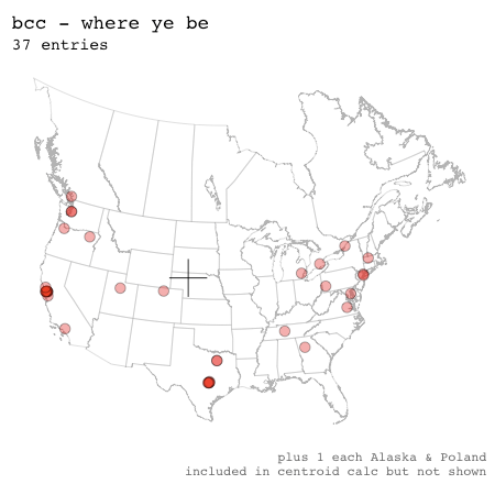
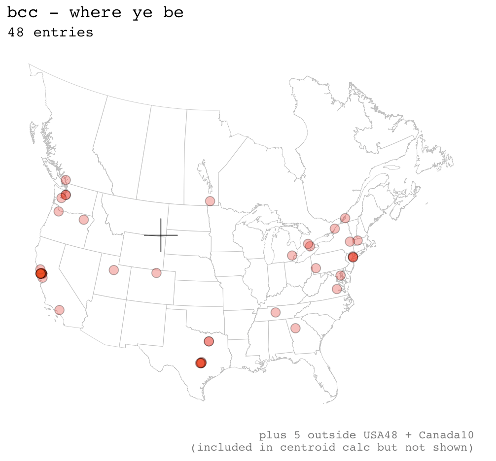
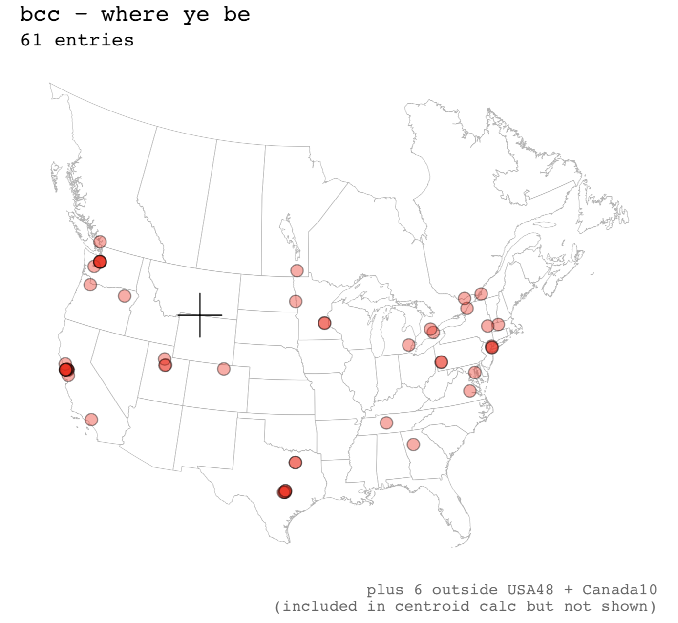
put some points on a map and calc centroid

.bcc_map.txt

just to rename gist

.gitignore

*.csv
*.pdf

1_map_data.R

setwd('~/Documents/personal/r_stuff/bcc_map/')

library(ggmap)
library(data.table)
library(tidyverse)
library(sf)
library(rnaturalearth)

fl_name <- 'map_data.csv'

# raw data
dat <-
"94619
75218
brockville ontario
91501
99507
94611
78704
80524
94103
94103
37064
95050
30303
10040
48154
Brantford, Ontario, Canada
94703
75218
78753
11222
78702
94608
97850
98122
78721
Seattle, WA, USA
78735
warsaw, poland
23224
vancouver
21401
84604
97202
94114
01351
94952
15219
Waterloo, ON
Montreal, QC
little diomede, AK
melbourne, au
98506
94105
94110
Helsinki, Finland
11106
12208
Steinbach, Manitoba, Canada
84101
Melbourne, Australia
Minneapolis, Minnesota, United States
84601
98103
78753
58103
98103
98119
15201
94102
Gatineau. Quebec, Canada
55407" %>%
  strsplit('\n') %>%
  unlist %>%
  tolower %>%
  data.table(loc_txt=.)

if(file.exists(fl_name)) {
  # we already have some geocoded results on disk. so load those...
  geo_result <- fread(fl_name)[, .(lon, lat)]
  #...and just geocode new ones
  more_geo_result <-
    (nrow(geo_result)+1):nrow(dat) %>%
    
    # geocoding. careful, this costs money & requires gmaps API key
    dat[., loc_txt] %>% geocode
  
  geo_result <- rbind(geo_result[, .(lon, lat)], more_geo_result)
  
} else {
  # we got bupkis, geocode all
  # geocoding. careful, this costs money & requires gmaps API key
  geo_result <- geocode(dat$loc_txt)
}
  
# collect geo strings and lat/lon together, write to disk
dat <- data.table(dat, geo_result)
write.csv(dat, fl_name, row.names = F)

2_points_on_map.R

# load rnaturalearth base map
base_map <- ne_states(
  country = c('united states of america','canada'),
  returnclass = 'sf')

my_crs <- 
  # lcc us/canada
  paste("+proj=lcc +lat_1=20 +lat_2=60 +lat_0=40 +lon_0=-96",
        "+x_0=0 +y_0=0 +ellps=GRS80 +datum=NAD83")
  # "+proj=vandg +lon_0=0 +x_0=0 +y_0=0 +R_A +ellps=WGS84 +datum=WGS84"

# subset to relevant map area, apply projection
base_map_proj <-
  filter(base_map,
         !postal %in% c('AK', 'HI', 'YT', 'NT', 'NU')) %>%
  sf::st_transform(my_crs)

sf_points <- 
  dat %>% 
  st_as_sf(coords = c('lon', 'lat'), crs=4326) %>%
  st_transform(crs = my_crs)

# calc centroid
spdf_points <- as(sf_points[, 'geometry'], 'Spatial')
spdf_points@data <- data.frame(weight=rep(1, nrow(sf_points)))
sf_center <- 
  spatialEco::wt.centroid(spdf_points, 'weight') %>% 
  st_as_sf
# print out as lat/lon
st_transform(sf_center, crs=4326)

# locs to omit
loc_omit <- filter(dat, lon > -72 | lon < -125)[['loc_txt']]

# draw map
ggplot() +
  geom_sf(data = base_map_proj,
          color = 'grey70', fill=NA, size=0.15) +
  geom_sf(data = filter(
    sf_points, 
    #!grepl('99507|poland|\\, ak$', loc_txt, ignore.case = T)
    !loc_txt %in% loc_omit
    ),
    alpha=0.4, shape=21, fill='red', size=3) +
  geom_sf(data=sf_center, color='black', shape=3, size=8) +
  labs(title='bcc - where ye be',
       subtitle = paste(nrow(dat), 'entries'),
       caption = paste0('plus ',length(loc_omit), ' outside USA48 + Canada10\n',
                        '(included in centroid calc but not shown)')) +
  theme_minimal(base_family = 'Courier') +
  theme(axis.text = element_blank(),
        plot.caption = element_text(color='grey40'),
        panel.grid.major = element_line(colour = "transparent"))

outname <- paste0('bcc_map_', nrow(dat), '.pdf')
ggsave(outname, w=7, h=5)