# from py to R ------------------------------------------------------------
# to convert the a python notebook to Rmd file
# with https://pkgs.rstudio.com/rmarkdown/reference/convert_ipynb.html
# for one sample ----------------------------------------------------------
set.seed(123)
rnorm(n = 25,mean = 100,sd = 20)
#> [1] 88.79049 95.39645 131.17417 101.41017 102.58575 134.30130 109.21832
#> [8] 74.69878 86.26294 91.08676 124.48164 107.19628 108.01543 102.21365
#> [15] 88.88318 135.73826 109.95701 60.66766 114.02712 90.54417 78.64353
#> [22] 95.64050 79.47991 85.42218 87.49921
# (1) generate multiple random samples ----------------------------------------
library(tidyverse)
# with https://gist.github.com/avallecam/ee009a8065921e74054935f87e3bf7d5
data <- tibble(
class = 1:10,
n = 25, # this changes
mean = 100,
sd = 20
) %>%
mutate(sample = pmap(select(., -class), rnorm))
data
#> # A tibble: 10 × 5
#> class n mean sd sample
#> <int> <dbl> <dbl> <dbl> <list>
#> 1 1 25 100 20 <dbl [25]>
#> 2 2 25 100 20 <dbl [25]>
#> 3 3 25 100 20 <dbl [25]>
#> 4 4 25 100 20 <dbl [25]>
#> 5 5 25 100 20 <dbl [25]>
#> 6 6 25 100 20 <dbl [25]>
#> 7 7 25 100 20 <dbl [25]>
#> 8 8 25 100 20 <dbl [25]>
#> 9 9 25 100 20 <dbl [25]>
#> 10 10 25 100 20 <dbl [25]>
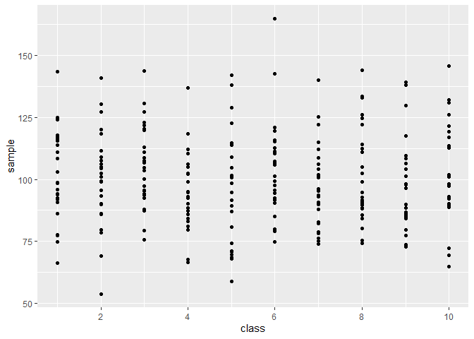
## distribution of values per sample ---------------------------------------
# with https://stackoverflow.com/questions/15622001/how-to-display-only-integer-values-on-an-axis-using-ggplot2
data %>%
select(class,sample) %>%
unnest(sample) %>%
ggplot(aes(x = class, y = sample)) +
geom_point() +
scale_x_continuous(breaks= scales::pretty_breaks())
## (2) create summary statistics per sample ------------------------------------

# with https://dplyr.tidyverse.org/articles/rowwise.html#motivation
data_summary <-
  data %>%
  select(class, sample) %>%
  rowwise() %>%
  mutate(s_mean = mean(sample),
         s_sd = sd(sample)) %>%
  ungroup()

data_summary
#> # A tibble: 10 × 4
#>    class sample     s_mean  s_sd
#>    <int> <list>      <dbl> <dbl>
#>  1     1 <dbl [25]>  102.   18.4
#>  2     2 <dbl [25]>  100.   19.4
#>  3     3 <dbl [25]>  106.   16.6
#>  4     4 <dbl [25]>   94.5  15.6
#>  5     5 <dbl [25]>   95.4  23.6
#>  6     6 <dbl [25]>  104.   19.8
#>  7     7 <dbl [25]>   97.2  17.0
#>  8     8 <dbl [25]>  102.   19.5
#>  9     9 <dbl [25]>   97.5  18.5
#> 10    10 <dbl [25]>  103.   20.1

## distribution of all summary statistics ----------------------------------

data_summary %>%
  ggplot(aes(x = s_mean)) +
  geom_histogram()
#> `stat_bin()` using `bins = 30`. Pick better value with `binwidth`.
## (3) variability of sample means ---------------------------------------------

data_summary %>%
  summarise(
    n_samples = n(),
    mean_s_mean = mean(s_mean),
    sd_s_mean = sd(s_mean))
#> # A tibble: 1 × 3
#>   n_samples mean_s_mean sd_s_mean
#>       <int>       <dbl>     <dbl>
#> 1        10        100.      3.89

# multiple samples for multiple sizes -------------------------------------

# with https://tidyr.tidyverse.org/reference/expand.html
expand_summary <-
  # (0) generate multiple combinations, instead of tibble
  expand_grid(
  n = c(10,25,50), # this changes
  class = 1:1000,
  mean = 100,
  sd = 20
) %>%
  # (1) generate multiple random samples
  mutate(sample = pmap(select(., -class), rnorm)) %>%
  # (2) create summary statistics per sample
  select(n, class, sample) %>%
  rowwise() %>%
  mutate(s_mean = mean(sample),
         s_sd = sd(sample)) %>%
  ungroup()

# distribution of all summary statistics
expand_summary %>%
  ggplot(aes(x = s_mean)) +
  geom_histogram() +
  facet_grid(~n)
#> `stat_bin()` using `bins = 30`. Pick better value with `binwidth`.
expand_summary %>%
  # (3) variability of sample means
  group_by(n) %>%
  summarise(
    n_samples = n(),
    mean_s_mean = mean(s_mean),
    sd_s_mean = sd(s_mean))
#> # A tibble: 3 × 4
#>       n n_samples mean_s_mean sd_s_mean
#>   <dbl>     <int>       <dbl>     <dbl>
#> 1    10      1000       100.       6.26
#> 2    25      1000        99.9      3.87
#> 3    50      1000       100.       2.77

# mean of sample means
# standard deviation of sample means ~ standard error
Created on 2023-11-13 with reprex v2.0.2
figure 1