AI Math

kmeans.md

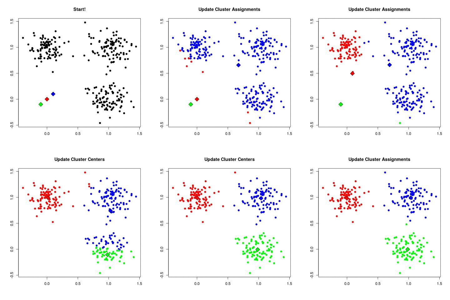
K-Means

• Unsupervised
• Determines the center of clusters
• Given how many clusters you want to find

When To Use

• Your data is numeric. It doesn't work with categorical features. We're computing the distance between real numbers!
• If you don't have labels for your data
• K-means is the simplest. To implement and to run. All you need to do is choose "k" and run it a number of times.
• K-means and other clustering algorithms shine when you have multivariate data. They will "work" with 1-dimensional data, but they are not very smart anymore.
• useful when you have an idea of how many clusters actually exists in your space.

Where it is used

• Security
• Classification
• Generally identifying something unknown

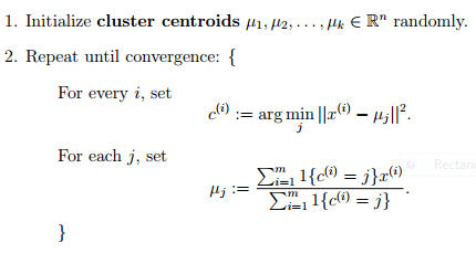
How it works

In other words

• Place all the points
• Place centroids in random location
• for each point assign to the nearest centroid

Centroid

Let P be any point in the plane of a triangle with vertices A, B, and C and centroid G. Then the sum of the squared distances of P from the three vertices exceeds the sum of the squared distances of the centroid G from the vertices by three times the squared distance between P and G:

The sum of the squares of the triangle's sides equals three times the sum of the squared distances of the centroid from the vertices:

Formula

Example

Code Example

import numpy as np
import matplotlib.pyplot as plt
import matplotlib.animation as animation

def load_dataset(name):
    return np.loadtxt(name)


def euclidian(a, b):
    return np.linalg.norm(a-b)


def plot(dataset, history_centroids, belongs_to):
    colors = ['r', 'g']

    fig, ax = plt.subplots()

    for index in range(dataset.shape[0]):
        instances_close = [i for i in range(len(belongs_to)) if belongs_to[i] == index]
        for instance_index in instances_close:
            ax.plot(dataset[instance_index][0], dataset[instance_index][1], (colors[index] + 'o'))

    history_points = []
    for index, centroids in enumerate(history_centroids):
        for inner, item in enumerate(centroids):
            if index == 0:
                history_points.append(ax.plot(item[0], item[1], 'bo')[0])
            else:
                history_points[inner].set_data(item[0], item[1])
                print("centroids {} {}".format(index, item))

                plt.pause(0.8)


def kmeans(k, epsilon=0, distance='euclidian'):
    history_centroids = []
    if distance == 'euclidian':
        dist_method = euclidian
    dataset = load_dataset('durudataset.txt')
    # dataset = dataset[:, 0:dataset.shape[1] - 1]
    num_instances, num_features = dataset.shape
    prototypes = dataset[np.random.randint(0, num_instances - 1, size=k)]
    history_centroids.append(prototypes)
    prototypes_old = np.zeros(prototypes.shape)
    belongs_to = np.zeros((num_instances, 1))
    norm = dist_method(prototypes, prototypes_old)
    iteration = 0
    while norm > epsilon:
        iteration += 1
        norm = dist_method(prototypes, prototypes_old)
        prototypes_old = prototypes
        for index_instance, instance in enumerate(dataset):
            dist_vec = np.zeros((k, 1))
            for index_prototype, prototype in enumerate(prototypes):
                dist_vec[index_prototype] = dist_method(prototype,
                                                        instance)

            belongs_to[index_instance, 0] = np.argmin(dist_vec)

        tmp_prototypes = np.zeros((k, num_features))

        for index in range(len(prototypes)):
            instances_close = [i for i in range(len(belongs_to)) if belongs_to[i] == index]
            prototype = np.mean(dataset[instances_close], axis=0)
            # prototype = dataset[np.random.randint(0, num_instances, size=1)[0]]
            tmp_prototypes[index, :] = prototype

        prototypes = tmp_prototypes

        history_centroids.append(tmp_prototypes)

    # plot(dataset, history_centroids, belongs_to)

    return prototypes, history_centroids, belongs_to


def execute():
    dataset = load_dataset('durudataset.txt')
    centroids, history_centroids, belongs_to = kmeans(2)
    plot(dataset, history_centroids, belongs_to)

execute()

0.196705753183788	0.266174967499455
0.413286989521383	0.355828352990633
0.338435546719209	0.435738258997923
0.103801517189990	0.164344805836115
0.159052363075132	0.325059012698889
0.0669054926780630	0.487418074001379
0.335731444739015	0.0379836806470678
0.285495537731203	0.293509583541386
0.0848835330132443	0.206943248886680
0.0738278885758684	0.154568213233134
0.238039859133728	0.131917020763398
0.454051208253475	0.379383132540102
0.276087513357917	0.497607990564876
0.0164699463749383	0.0932857220706846
0.0269314632177781	0.390572634267382
0.402531614279451	0.0978989905133660
0.225687427351724	0.496179486589963
0.191323114779979	0.401130784882144
0.394821851844845	0.212113354951653
0.182143434749897	0.364431934025687
1.49835358252355	1.40350138880436
1.80899026719904	1.93497908617805
1.35650893348105	1.47948454563248
1.07324343448981	1.23179161166312
1.59099145527485	1.39629024850978
1.91018783072814	1.70507747511279
1.19376593616661	1.55855903456055
1.43236779153440	1.75663070089437
1.74915972906801	1.99548105855526
1.03918448664758	1.96243140436663
1.94632498980548	1.53506710525616
1.76367332366376	1.96387012997171
1.55882055050956	1.11562587918126
1.18384294446577	1.05144829323021
1.49794881501895	1.30434894563657
1.51784560023405	1.58019183314271
1.99424301064405	1.53096445233828
1.85485168309068	1.90120809265314
1.96240393971197	1.54055042517024
1.67894100897703	1.43198061085668

neural.md

• Classification
  • SVM
  • KNN
  • CART
• Regression
  • CART
  • LASSO
  • Linear Regression
• Cluster Analysis
  • K-Means
  • Heirarchical Clustering
• Dimensionality Reduction
  • ICA PCA

regression.md

Linear

One of the strongest mainstays of statistics is the linear model. That is, when there aren’t any known relationships among the observed data, the simplest possible relationship one could discover is a linear one. A change in corresponds to a proportional change in , and so one could hope there exist constants so that (as random variables) .  If this were the case then we could just draw many pairs of sample values of and , and try to estimate the value of and .

If the data actually lies on a line, then two sample points will be enough to get a perfect prediction. Of course, nothing is exact outside of mathematics. And so if we were to use data coming from the real world, and even if we were to somehow produce some constants , our “predictor” would almost always be off by a bit. In the diagram below, where it’s clear that the relationship between the variables is linear, only a small fraction of the data points appear to lie on the line itself.

In such scenarios it would be hopelessly foolish to wish for a perfect predictor, and so instead we wish to summarize the trends in the data using a simple description mechanism. In this case, that mechanism is a line. Now the computation required to find the “best” coefficients of the line is quite straightforward once we pick a suitable notion of what “best” means.

Now suppose that we call our (presently unknown) prediction function . We often call the function we’re producing as a result of our learning algorithm the hypothesis, but in this case we’ll stick to calling it a prediction function. If we’re given a data point where is a value of and of , then the error of our predictor on this example is . Geometrically this is the vertical distance from the actual value to our prediction for the same , and so we’d like to minimize this error. Indeed, we’d like to minimize the sum of all the errors of our linear predictor over all data points we see. We’ll describe this in more detail momentarily.

The word “minimize” might evoke long suppressed memories of torturous Calculus lessons, and indeed we will use elementary Calculus to find the optimal linear predictor. But one small catch is that our error function, being an absolute value, is not differentiable! To mend this we observe that minimizing the absolute value of a number is the same as minimizing the square of a number. In fact, , and the square root function and its inverse are both increasing functions; they preserve minima of sets of nonnegative numbers.  So we can describe our error as , and use calculus to our heart’s content.

Which can also be written as

Note that since we’re fixing our data sample, the function is purely a function of the variables . Now we want to minimize this quantity with respect to , so we can take a gradient,

Note that since we’re fixing our data sample, the function is purely a function of the variables . Now we want to minimize this quantity with respect to , so we can take a gradient,

and set them simultaneously equal to zero. In the first we solve for :

If we denote by this is just . Substituting into the other equation we get

Which, by factoring out , further simplifies to

And so

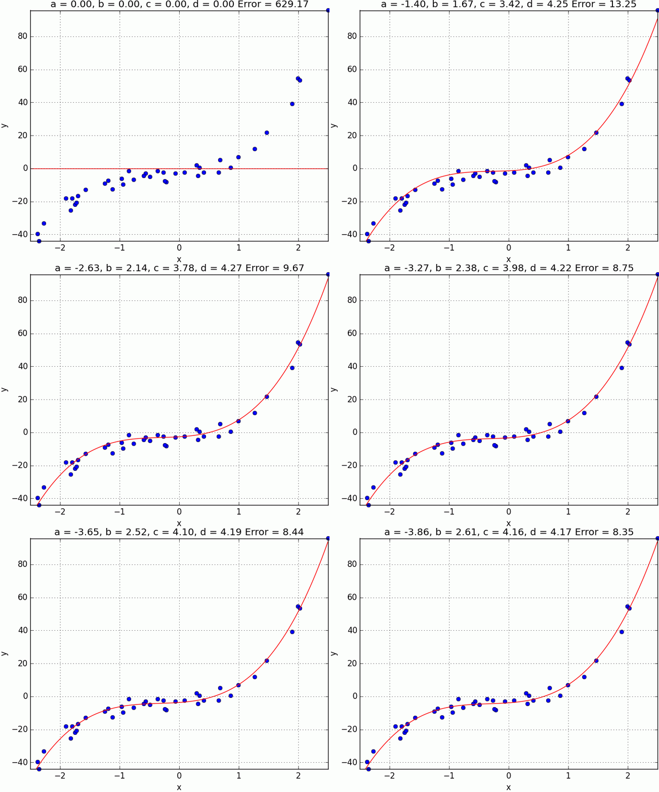
Nonlinear Example

Sample Code

from numpy import *
import matplotlib.pyplot as plt

# y = mx+c

def compute_error_for_given_points(c, m, points):
    totalError = 0

    for i in range(0, len(points)):
        x = points[i, 0]
        y = points[i, 1]
        totalError += (y - (m*x+c)) ** 2
    return totalError / float(len(points))

def step_gradient(c_current, m_current, points, learning_rate):
    #gradient descent
    c_gradient = 0
    m_gradient = 0
    N= float(len(points))

    for i in range(0, len(points)):
        x = points[i, 0]
        y = points[i, 1]
        c_gradient += -(2/N) * (y - ((m_current * x) + c_current))
        m_gradient += -(2/N) * x * (y - ((m_current * x) + c_current))
    new_c = c_current - (learning_rate * c_gradient)
    new_m = m_current - (learning_rate * m_gradient)
    return [new_c, new_m]

def gradient_descent_runner(points, starting_c, starting_m, learning_rate, num_iterations):
    c = starting_c
    m = starting_m

    for i in range(num_iterations):
        c, m = step_gradient(c, m, array(points), learning_rate)
    return [c,m]

def run():
    points = genfromtxt('data/live_data.csv', delimiter=',')
    #hyperparameters
    learning_rate = 0.0002
    initial_c = 0
    initial_m = 0
    num_iterations = 1000

    print("Starting gradient descent at c={0}, m={1}, error={2}".format(initial_c, initial_m, compute_error_for_given_points(initial_c, initial_m, points)))
    print("Running...")
    [c, m] = gradient_descent_runner(points, initial_c, initial_m, learning_rate, num_iterations)
    print("After {0} iterations c={1}, m={2}, error={3}".format(num_iterations, c, m, compute_error_for_given_points(c, m, points)))

    #plot of points and regression line
    plt.scatter(points[:, 0], points[:, 1])
    plt.plot(points[:, 0], (points[:,0]*m)+c)
    plt.show()

if __name__ == '__main__':
    run()

svm.md

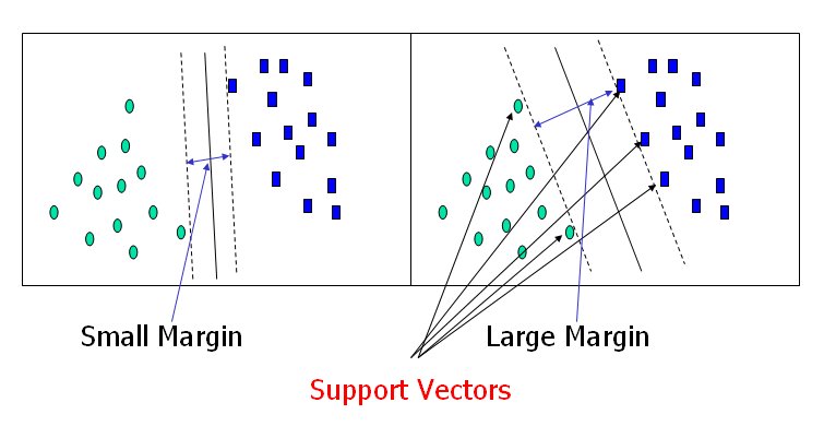
Support Vector Machines

• Supervised
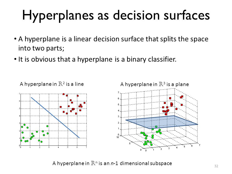
• Determines a hyperplane

When To Use

• Binary Decision
• Data set is small

Hyperplanes

Non Linear Hyperplanes

Loss function

We'll use the Hinge loss. This is a loss function used for training classifiers. The hinge loss is used for "maximum-margin" classification, most notably for support vector machines (SVMs).

c is the loss function, x the sample, y is the true label, f(x) the predicted label.

Objective Function

As you can see, our objective of a SVM consists of two terms. The first term is a regularizer, the heart of the SVM, the second term the loss. The regularizer balances between margin maximization and loss. We want to find the decision surface that is maximally far away from any data points.

How do we minimize our loss/optimize for our objective (i.e learn)?

We have to derive our objective function to get the gradients! Gradient descent ftw. As we have two terms, we will derive them seperately using the sum rule in differentiation.

This means, if we have a misclassified sample, we update the weight vector w using the gradients of both terms, else if classified correctly,we just update w by the gradient of the regularizer.

Misclassification condition

Update rule for our weights (misclassified)

including the learning rate η and the regularizer λ The learning rate is the length of the steps the algorithm makes down the gradient on the error curve.

• Learning rate too high? The algorithm might overshoot the optimal point.
• Learning rate too low? Could take too long to converge. Or never converge.

The regularizer controls the trade off between the achieving a low training error and a low testing error that is the ability to generalize your classifier to unseen data. As a regulizing parameter we choose 1/epochs, so this parameter will decrease, as the number of epochs increases.

• Regularizer too high? overfit (large testing error)
• Regularizer too low? underfit (large training error)

Update rule for our weights (correctly classified)

Example

Code Example

import numpy as np
import matplotlib.pyplot as plt
from matplotlib import style
from sklearn import svm
style.use("ggplot")

#points
X = np.array([
    [1,2],
    [5,8],
    [1.5,1.8],
    [8,8],
    [1,0.6],
    [9,11]]
)

#labels
y = [0, 1, 0, 1, 0, 1]

#classifier
clf = svm.SVC(kernel='linear', C = 1.0)
clf.fit(X,y)

#prediction
print(clf.predict([[10.58, 10.76]]))

#coefficient
w = clf.coef_[0]
print(w)

#draw it
a = -w[0] / w[1]

xx = np.linspace(0,12)
yy = a * xx - clf.intercept_[0] / w[1]

h0 = plt.plot(xx, yy, 'k-', label="non weighted div")

plt.scatter(X[:, 0], X[:, 1], c = y)
plt.legend()
plt.show()