
Last active
February 3, 2022 17:16
-
-
Save ctesta01/7d4d73f6fc6c353d4da867d9d1a21a37 to your computer and use it in GitHub Desktop.
Using consistent color scales across different plots with scale_color_gradient
This file contains hidden or bidirectional Unicode text that may be interpreted or compiled differently than what appears below. To review, open the file in an editor that reveals hidden Unicode characters.
Learn more about bidirectional Unicode characters
| library(palmerpenguins) | |
| library(purrr) | |
| library(ggplot2) | |
| library(dplyr) | |
| library(patchwork) | |
| # let's say I want to show bill_length_mm across different species (one plot for each species), | |
| # but each plot should have the same color scale | |
| # one common issue is that if you just use scale_color_gradient() or scale_color_brewer(), each | |
| # of your plots will be shown with a color gradient palette that suits the data in that plot -- | |
| # with its own unique min/max range. | |
| # | |
| # if we're trying to compare the same variable in multiple plots, it can be important to | |
| # standardize the legend on the color scale. | |
| # | |
| # this is a simple example script showing how to do this with across 3 figures using the | |
| # palmerpenguins dataset, patchwork (for the layout), and purrr (to produce multiple plots in | |
| # functional programming style). | |
| # specify color scale -- in this case i'm using viridis::magma so that | |
| # the color palette should be colorblind friendly. | |
| viridis_5 <- viridis::magma(n=5, end = .8) | |
| high <- viridis_5[4] | |
| low <- viridis_5[2] | |
| # observe range overall | |
| range_observed_length <- range(penguins$bill_length_mm, na.rm=T) | |
| range_observed_depth <- range(penguins$bill_depth_mm, na.rm=T) | |
| # calculate cutpoints | |
| cutpoints <- seq(range_observed_length[1], range_observed_length[2], length.out = 5) | |
| # construct multiple ggplots with the same scale_color_gradient | |
| ggplots <- purrr::map( | |
| unique(penguins$species), | |
| ~ filter(penguins, species == .)) %>% | |
| purrr::map( | |
| ~ ggplot(., aes( | |
| x = bill_length_mm, | |
| y = bill_depth_mm, | |
| color = bill_length_mm)) + | |
| geom_point() + | |
| expand_limits(x = range_observed_length, y = range_observed_depth) + | |
| scale_color_gradient( | |
| low = low, | |
| high = high, | |
| breaks = cutpoints, | |
| limits = range_observed_length)) | |
| # give them each appropriate titles | |
| ggplots[[1]] <- ggplots[[1]] + ggtitle("Bill Length (mm) Relationship to Bill Depth", "Adelie Penguins") | |
| ggplots[[2]] <- ggplots[[2]] + ggtitle("Bill Length (mm) Relationship to Bill Depth", "Gentoo Penguins") | |
| ggplots[[3]] <- ggplots[[3]] + ggtitle("Bill Length (mm) Relationship to Bill Depth", "Chinstrap Penguins") | |
| # create a patchwork layout | |
| ggplots[[1]] + ggplots[[2]] / ggplots[[3]] | |
| # render to image | |
| ggsave("example.png", width = 12, height = 8) |

Author
Here's an example using scale_color_gradient2 –– remember that you have to specify the midpoint argument if it's not 0 in scale_color_gradient2.
library(palmerpenguins)
library(purrr)
library(ggplot2)
library(dplyr)
library(patchwork)

# let's say I want to show bill_length_mm across different species (one plot for each species),
# but each plot should have the same color scale

# one common issue is that if you just use scale_color_gradient() or scale_color_brewer(), each
# of your plots will be shown with a color gradient palette that suits the data in that plot --
# with its own unique min/max range.
#
# if we're trying to compare the same variable in multiple plots, it can be important to
# standardize the legend on the color scale.
#
# this is a simple example script showing how to do this with across 3 figures using the
# palmerpenguins dataset, patchwork (for the layout), and purrr (to produce multiple plots in
# functional programming style).

# specify color scale -- in this case i'm using viridis::magma so that
# the color palette should be colorblind friendly.
viridis_5 <- viridis::magma(n=5, end = .8)
high <- viridis_5[4]
mid <- viridis_5[3]
low <- viridis_5[2]

# observe range overall
range_observed_length <- range(penguins$bill_length_mm, na.rm=T)
range_observed_depth <- range(penguins$bill_depth_mm, na.rm=T)

# calculate cutpoints
cutpoints <- seq(range_observed_length[1], range_observed_length[2], length.out = 5)

# construct multiple ggplots with the same scale_color_gradient
ggplots <- purrr::map(
  unique(penguins$species),
  ~ filter(penguins, species == .)) %>%
  purrr::map(
  ~ ggplot(., aes(
    x = bill_length_mm,
    y = bill_depth_mm,
    color = bill_length_mm)) +
    geom_point() +
    expand_limits(x = range_observed_length, y = range_observed_depth) +
    scale_color_gradient2(
      low = low,
      mid = mid,
      high = high,
      midpoint = mean(range_observed_length),
      breaks = cutpoints,
      limits = range_observed_length))

# give them each appropriate titles
ggplots[[1]] <- ggplots[[1]] + ggtitle("Bill Length (mm) Relationship to Bill Depth", "Adelie Penguins")
ggplots[[2]] <- ggplots[[2]] + ggtitle("Bill Length (mm) Relationship to Bill Depth", "Gentoo Penguins")
ggplots[[3]] <- ggplots[[3]] + ggtitle("Bill Length (mm) Relationship to Bill Depth", "Chinstrap Penguins")

# create a patchwork layout
ggplots[[1]] + ggplots[[2]] / ggplots[[3]]

# render to image
ggsave("example.png", width = 12, height = 8)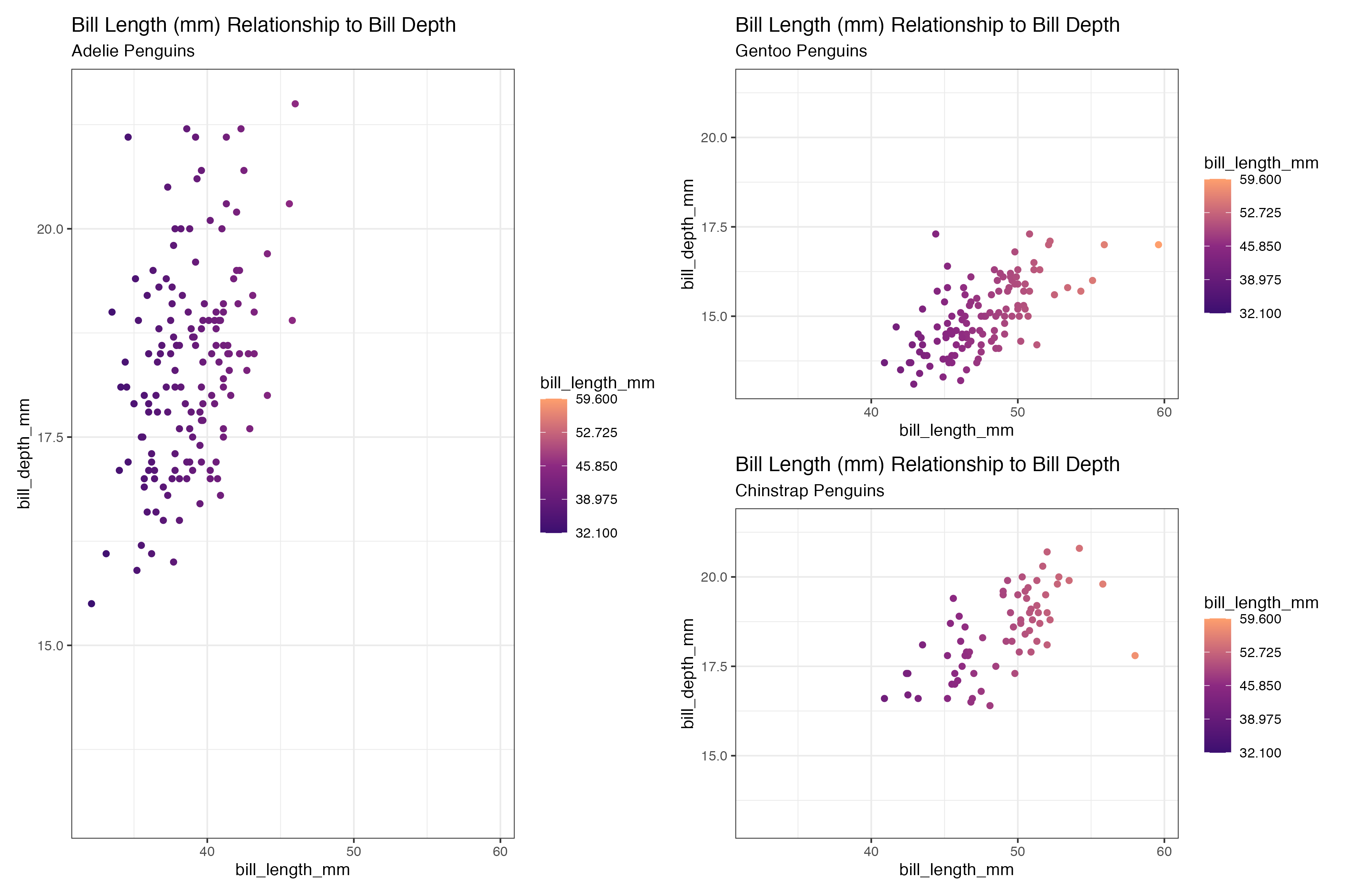
Sign up for free
to join this conversation on GitHub.
Already have an account?
Sign in to comment
Uh oh!
There was an error while loading. Please reload this page.