rm(list = ls())
initrun <- Sys.time()
#Implementation of head/tails 1.0
#1. Characterization of heavy-tail distributions----
set.seed(1234)
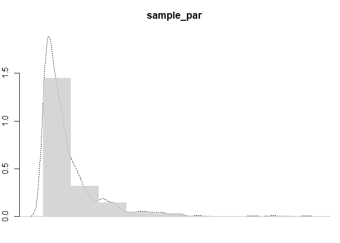
#Pareto distribution a=2 b=6 n=1000
sample_par <- 2 / (1 - runif(1000)) ^ (1 / 6)
cols <- adjustcolor("grey80", alpha.f = 0.8)
opar <- par(no.readonly = TRUE)
par(mar = c(2, 2, 3, 1))
#Figures
plot(
density(sample_par),
lty = 3,
axes = FALSE,
ylab = "",
xlab = "",
main = "sample_par"
)
axis(2)
hist(
sample_par,
col = cols,
border = NA,
main = "Pareto",
freq = FALSE,
axes = FALSE,
add = TRUE
)
#2. Step by step example----
set.seed(1234)
sample_par <- 2 / (1 - runif(1000)) ^ (1 / 6)
var <- sample_par
thr <- 0.35 #Cherry-picked thresold  for the example

#Step1
mu0 <- mean(var)
#The breaks are the means of the head
breaks <- c(mu0)
n0 <- length(var)
head0 <- var[var > mu0]
prop0 <- length(head0) / n0

plot(
  density(var),
  lty = 3,
  ylab = "",
  xlab = "",
  main = "Iter1"
)
abline(v = mu0, col = "red")
text(x = 6,
     y = 1,
     labels = paste0("PropHead: ", round(prop0, 4)))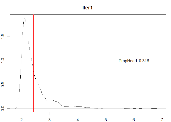
prop0 <= thr &
  n0 > 1 #Additional control to stop if no more breaks are possible
#> [1] TRUE


#The process is iterative through the head, i.e, now var <- head0
var <- head0

#Iter2
mu1 <- mean(var)
#Add the break
breaks <- c(breaks, mu1)
n1 <- length(var)
head1 <- var[var > mu1]
prop1 <- length(head1) / n1

plot(
  density(var),
  lty = 3,
  ylab = "",
  xlab = "",
  main = "Iter2"
)
abline(v = mu1, col = "red")
text(x = 6,
     y = 1,
     labels = paste0("PropHead: ", round(prop1, 4)))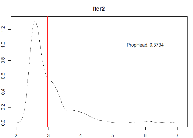
prop1 <= thr  & n1 > 1
#> [1] FALSE

# End given that condition is FALSE

#Summary
summiter <- data.frame(
  iter = c(1, 2),
  n = c(n0, n1),
  nhead = c(length(head0), length(head1)),
  mu = c(mu0, mu1),
  prophead = c(prop0, prop1)
)
summiter$breaks <- breaks
knitr::kable(summiter, format = "markdown")
| iter |
n |
nhead |
mu |
prophead |
breaks |
| 1 |
1000 |
316 |
2.422568 |
0.3160000 |
2.422568 |
| 2 |
316 |
118 |
2.971249 |
0.3734177 |
2.971249 |
#3. Standalone function----
# Default thresold = 0.4 as per Jiang et al. (2013)
ht_index <- function(var, style = "headtails", ...) {
if (style == "headtails") {
# Contributed Diego Hernangomez
dots <- list(...)
thr = ifelse(is.null(dots$thr),
.4,
dots$thr)
thr <- min(1,max(0, thr))
head <- var
breaks <- NULL #Init on null
#Safe-check loop to set a maximum of iterations
#Option to set a WHILE loop and set an additional par to stop the loop
for (i in 1:100) {
mu <- mean(head, na.rm = TRUE)
breaks <- c(breaks, mu)
ntot <- length(head)
#Switch head
head <- head[head > mu]
prop <- length(head) / ntot
keepiter <- prop <= thr & length(head) > 1
print(paste0("prop:", prop, " nhead:", length(head)))
if (isFALSE(keepiter)) {
#Just for checking the execution
# to remove on implementation
print(paste("Breaks found: ", i, ", Intervals:", i+1))
break
}
}
#Add min and max to complete intervals
breaks <- sort(unique(c(
min(var, na.rm = TRUE),
breaks,
max(var, na.rm = TRUE)
)))
#Remove on implementation
print(breaks)
return(breaks)
}
}
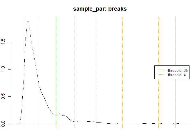
plot(
density(sample_par),
lty = 3,
axes = FALSE,
ylab = "",
xlab = "",
main = "sample_par: breaks"
)
axis(2)
abline(v = ht_index(sample_par, thr = 0.35), col = "green")
#> [1] "prop:0.316 nhead:316"
#> [1] "prop:0.373417721518987 nhead:118"
#> [1] "Breaks found: 2 , Intervals: 3"
#> [1] 2.000114 2.422568 2.971249 6.716770
abline(
v = ht_index(sample_par, thr = 0.4),
col = "orange",
lty = 3,
lwd = 0.5
)
#> [1] "prop:0.316 nhead:316"
#> [1] "prop:0.373417721518987 nhead:118"
#> [1] "prop:0.355932203389831 nhead:42"
#> [1] "prop:0.285714285714286 nhead:12"
#> [1] "prop:0.333333333333333 nhead:4"
#> [1] "prop:0.25 nhead:1"
#> [1] "Breaks found: 6 , Intervals: 7"
#> [1] 2.000114 2.422568 2.971249 3.559716 4.227112 5.055604 6.181099 6.716770
legend(
"right",
legend = c("thresold .35", "thresold .4"),
col = c("green", "orange"),
lty = c(1, 3),
cex = 0.8
)
#4. Test and stress----
#Init table on default
testresults <- data.frame(
  Title = NA,
  nsample  = NA,
  thresold = NA,
  nbreaks = NA,
  time_secs = NA
)

benchmarkdist <-
  function(dist,
           thr = 0.4,
           title = "",
           plot = TRUE) {
    dist = c(na.omit(dist))
    init <- Sys.time()
    br <- ht_index(dist, thr = thr)
    a <- Sys.time() - init
    print(a)
    test <- data.frame(
      Title = title,
      nsample  = format(length(dist), scientific = FALSE, big.mark = ","),
      thresold = thr,
      nbreaks = length(br) - 1,
      time_secs = as.character(a)
    )
    testresults <- unique(rbind(testresults, test))

    if (plot) {
      plot(density(dist),
           col = "black",
           main = paste0(title, ", thr =", thr, ", nbreaks = ", length(br)-1))
      abline(v = br,
             col = "green",
             lty = 3)
    }
    return(testresults)
  }


#Scalability: 5 millions
set.seed(2389)

#Pareto distributions a=7 b=14
paretodist <- 7 / (1 - runif(5000000)) ^ (1 / 14)
#Exponential dist
expdist <- rexp(5000000)
#Lognorm
lognormdist <- rlnorm(5000000)
#Weibull
weibulldist <- rweibull(5000000, 1, scale = 5)
#Normal dist
normdist <- rnorm(5000000)
#Left-tailed distr
leftnorm <- rep(normdist[normdist < mean(normdist)], 2)
#LogCauchy "super-heavy tail"
logcauchdist <- exp(rcauchy(5000000, 2, 4))
#Remove Inf - this check is already implemented on classIntervals
logcauchdist <- logcauchdist[logcauchdist < Inf]

#Tests
testresults <- benchmarkdist(paretodist, title = "Pareto Dist")
#> [1] "prop:0.3543272 nhead:1771636"
#> [1] "prop:0.354200862931212 nhead:627515"
#> [1] "prop:0.354158864728333 nhead:222240"
#> [1] "prop:0.354063174946004 nhead:78687"
#> [1] "prop:0.35352726625745 nhead:27818"
#> [1] "prop:0.355345459774247 nhead:9885"
#> [1] "prop:0.355791603439555 nhead:3517"
#> [1] "prop:0.35371054876315 nhead:1244"
#> [1] "prop:0.343247588424437 nhead:427"
#> [1] "prop:0.346604215456674 nhead:148"
#> [1] "prop:0.371621621621622 nhead:55"
#> [1] "prop:0.327272727272727 nhead:18"
#> [1] "prop:0.388888888888889 nhead:7"
#> [1] "prop:0.142857142857143 nhead:1"
#> [1] "Breaks found:  14 , Intervals: 15"
#>  [1]  7.000000  7.538849  8.119161  8.743518  9.416418 10.143382 10.929898
#>  [8] 11.777121 12.679457 13.651872 14.734872 15.963453 17.311978 18.988971
#> [15] 20.211755 23.807530
#> Time difference of 0.419203 secs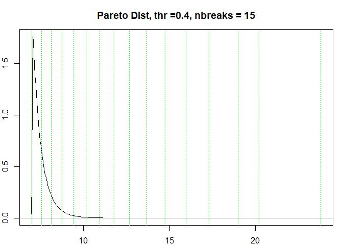
testresults <-
benchmarkdist(paretodist, 0, title = "Pareto Dist", plot = FALSE)
#> [1] "prop:0.3543272 nhead:1771636"
#> [1] "Breaks found: 1 , Intervals: 2"
#> [1] 7.000000 7.538849 23.807530
#> Time difference of 0.335701 secs
testresults <-
benchmarkdist(paretodist, 1, title = "Pareto Dist", plot = FALSE)
#> [1] "prop:0.3543272 nhead:1771636"
#> [1] "prop:0.354200862931212 nhead:627515"
#> [1] "prop:0.354158864728333 nhead:222240"
#> [1] "prop:0.354063174946004 nhead:78687"
#> [1] "prop:0.35352726625745 nhead:27818"
#> [1] "prop:0.355345459774247 nhead:9885"
#> [1] "prop:0.355791603439555 nhead:3517"
#> [1] "prop:0.35371054876315 nhead:1244"
#> [1] "prop:0.343247588424437 nhead:427"
#> [1] "prop:0.346604215456674 nhead:148"
#> [1] "prop:0.371621621621622 nhead:55"
#> [1] "prop:0.327272727272727 nhead:18"
#> [1] "prop:0.388888888888889 nhead:7"
#> [1] "prop:0.142857142857143 nhead:1"
#> [1] "Breaks found: 14 , Intervals: 15"
#> [1] 7.000000 7.538849 8.119161 8.743518 9.416418 10.143382 10.929898
#> [8] 11.777121 12.679457 13.651872 14.734872 15.963453 17.311978 18.988971
#> [15] 20.211755 23.807530
#> Time difference of 0.3962889 secs
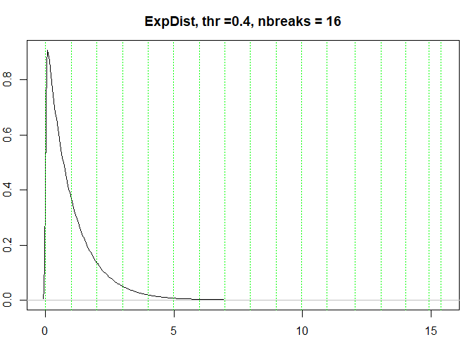
testresults <- benchmarkdist(expdist, title = "ExpDist")
#> [1] "prop:0.3677448 nhead:1838724"
#> [1] "prop:0.367977466982538 nhead:676609"
#> [1] "prop:0.368261433117207 nhead:249169"
#> [1] "prop:0.367794549081146 nhead:91643"
#> [1] "prop:0.367807688530493 nhead:33707"
#> [1] "prop:0.368706796807785 nhead:12428"
#> [1] "prop:0.36562600579337 nhead:4544"
#> [1] "prop:0.36949823943662 nhead:1679"
#> [1] "prop:0.363311494937463 nhead:610"
#> [1] "prop:0.360655737704918 nhead:220"
#> [1] "prop:0.354545454545455 nhead:78"
#> [1] "prop:0.397435897435897 nhead:31"
#> [1] "prop:0.387096774193548 nhead:12"
#> [1] "prop:0.333333333333333 nhead:4"
#> [1] "prop:0.5 nhead:2"
#> [1] "Breaks found: 15 , Intervals: 16"
#> [1] 4.534944e-07 9.990109e-01 1.998383e+00 2.996829e+00 3.993308e+00
#> [6] 4.988082e+00 5.985162e+00 6.973514e+00 7.969093e+00 8.968558e+00
#> [11] 9.974569e+00 1.096586e+01 1.203901e+01 1.307891e+01 1.402431e+01
#> [16] 1.493760e+01 1.539196e+01
#> Time difference of 0.3416569 secs
testresults <-
benchmarkdist(expdist, 0, title = "ExpDist", plot = FALSE)
#> [1] "prop:0.3677448 nhead:1838724"
#> [1] "Breaks found: 1 , Intervals: 2"
#> [1] 4.534944e-07 9.990109e-01 1.539196e+01
#> Time difference of 0.2051849 secs
testresults <-
benchmarkdist(expdist, 1, title = "ExpDist", plot = FALSE)
#> [1] "prop:0.3677448 nhead:1838724"
#> [1] "prop:0.367977466982538 nhead:676609"
#> [1] "prop:0.368261433117207 nhead:249169"
#> [1] "prop:0.367794549081146 nhead:91643"
#> [1] "prop:0.367807688530493 nhead:33707"
#> [1] "prop:0.368706796807785 nhead:12428"
#> [1] "prop:0.36562600579337 nhead:4544"
#> [1] "prop:0.36949823943662 nhead:1679"
#> [1] "prop:0.363311494937463 nhead:610"
#> [1] "prop:0.360655737704918 nhead:220"
#> [1] "prop:0.354545454545455 nhead:78"
#> [1] "prop:0.397435897435897 nhead:31"
#> [1] "prop:0.387096774193548 nhead:12"
#> [1] "prop:0.333333333333333 nhead:4"
#> [1] "prop:0.5 nhead:2"
#> [1] "prop:0.5 nhead:1"
#> [1] "Breaks found: 16 , Intervals: 17"
#> [1] 4.534944e-07 9.990109e-01 1.998383e+00 2.996829e+00 3.993308e+00
#> [6] 4.988082e+00 5.985162e+00 6.973514e+00 7.969093e+00 8.968558e+00
#> [11] 9.974569e+00 1.096586e+01 1.203901e+01 1.307891e+01 1.402431e+01
#> [16] 1.493760e+01 1.536455e+01 1.539196e+01
#> Time difference of 0.422025 secs
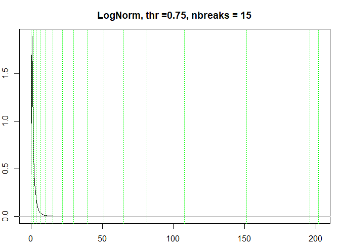
testresults <- benchmarkdist(lognormdist, 0.75, title = "LogNorm")
#> [1] "prop:0.3087264 nhead:1543632"
#> [1] "prop:0.309735740124589 nhead:478118"
#> [1] "prop:0.315926193952121 nhead:151050"
#> [1] "prop:0.319311486262827 nhead:48232"
#> [1] "prop:0.323270857521977 nhead:15592"
#> [1] "prop:0.333760903027193 nhead:5204"
#> [1] "prop:0.329554189085319 nhead:1715"
#> [1] "prop:0.332361516034985 nhead:570"
#> [1] "prop:0.335087719298246 nhead:191"
#> [1] "prop:0.350785340314136 nhead:67"
#> [1] "prop:0.26865671641791 nhead:18"
#> [1] "prop:0.277777777777778 nhead:5"
#> [1] "prop:0.4 nhead:2"
#> [1] "prop:0.5 nhead:1"
#> [1] "Breaks found: 14 , Intervals: 15"
#> [1] 5.960499e-03 1.648513e+00 3.693475e+00 6.541902e+00 1.037196e+01
#> [6] 1.539770e+01 2.186603e+01 2.976225e+01 3.948552e+01 5.107634e+01
#> [11] 6.517331e+01 8.141691e+01 1.075394e+02 1.514656e+02 1.960593e+02
#> [16] 2.019891e+02
#> Time difference of 0.3683128 secs
testresults <-
benchmarkdist(lognormdist, 0, title = "LogNorm", plot = FALSE)
#> [1] "prop:0.3087264 nhead:1543632"
#> [1] "Breaks found: 1 , Intervals: 2"
#> [1] 5.960499e-03 1.648513e+00 2.019891e+02
#> Time difference of 0.1818058 secs
testresults <-
benchmarkdist(lognormdist, 1, title = "LogNorm", plot = FALSE)
#> [1] "prop:0.3087264 nhead:1543632"
#> [1] "prop:0.309735740124589 nhead:478118"
#> [1] "prop:0.315926193952121 nhead:151050"
#> [1] "prop:0.319311486262827 nhead:48232"
#> [1] "prop:0.323270857521977 nhead:15592"
#> [1] "prop:0.333760903027193 nhead:5204"
#> [1] "prop:0.329554189085319 nhead:1715"
#> [1] "prop:0.332361516034985 nhead:570"
#> [1] "prop:0.335087719298246 nhead:191"
#> [1] "prop:0.350785340314136 nhead:67"
#> [1] "prop:0.26865671641791 nhead:18"
#> [1] "prop:0.277777777777778 nhead:5"
#> [1] "prop:0.4 nhead:2"
#> [1] "prop:0.5 nhead:1"
#> [1] "Breaks found: 14 , Intervals: 15"
#> [1] 5.960499e-03 1.648513e+00 3.693475e+00 6.541902e+00 1.037196e+01
#> [6] 1.539770e+01 2.186603e+01 2.976225e+01 3.948552e+01 5.107634e+01
#> [11] 6.517331e+01 8.141691e+01 1.075394e+02 1.514656e+02 1.960593e+02
#> [16] 2.019891e+02
#> Time difference of 0.392143 secs
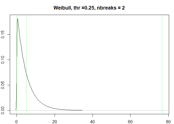
testresults <- benchmarkdist(weibulldist, 0.25, title = "Weibull")
#> [1] "prop:0.3679468 nhead:1839734"
#> [1] "Breaks found: 1 , Intervals: 2"
#> [1] 2.735760e-07 5.001702e+00 7.673301e+01
#> Time difference of 0.3522601 secs
testresults <-
benchmarkdist(weibulldist, 0, title = "Weibull", plot = FALSE)
#> [1] "prop:0.3679468 nhead:1839734"
#> [1] "Breaks found: 1 , Intervals: 2"
#> [1] 2.735760e-07 5.001702e+00 7.673301e+01
#> Time difference of 0.2157819 secs
testresults <-
benchmarkdist(weibulldist, 1, title = "Weibull", plot = FALSE)
#> [1] "prop:0.3679468 nhead:1839734"
#> [1] "prop:0.367591727934582 nhead:676271"
#> [1] "prop:0.367926467348149 nhead:248818"
#> [1] "prop:0.367995884542115 nhead:91564"
#> [1] "prop:0.367447905290289 nhead:33645"
#> [1] "prop:0.368108188438104 nhead:12385"
#> [1] "prop:0.373112636253533 nhead:4621"
#> [1] "prop:0.357714780350573 nhead:1653"
#> [1] "prop:0.372655777374471 nhead:616"
#> [1] "prop:0.375 nhead:231"
#> [1] "prop:0.350649350649351 nhead:81"
#> [1] "prop:0.37037037037037 nhead:30"
#> [1] "prop:0.366666666666667 nhead:11"
#> [1] "prop:0.363636363636364 nhead:4"
#> [1] "prop:0.5 nhead:2"
#> [1] "prop:0.5 nhead:1"
#> [1] "Breaks found: 16 , Intervals: 17"
#> [1] 2.735760e-07 5.001702e+00 1.000405e+01 1.501010e+01 2.001468e+01
#> [6] 2.501961e+01 3.004452e+01 3.504632e+01 3.991777e+01 4.495168e+01
#> [11] 4.986135e+01 5.441215e+01 5.900803e+01 6.358776e+01 6.870115e+01
#> [16] 7.444729e+01 7.666662e+01 7.673301e+01
#> Time difference of 0.4132988 secs
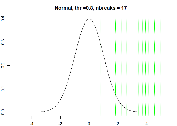
testresults <- benchmarkdist(normdist, 0.8, title = "Normal")
#> [1] "prop:0.5001914 nhead:2500957"
#> [1] "prop:0.425015304141575 nhead:1062945"
#> [1] "prop:0.404747188236456 nhead:430224"
#> [1] "prop:0.39417373275317 nhead:169583"
#> [1] "prop:0.390198309972108 nhead:66171"
#> [1] "prop:0.386498617219023 nhead:25575"
#> [1] "prop:0.380879765395894 nhead:9741"
#> [1] "prop:0.380043116723129 nhead:3702"
#> [1] "prop:0.388438681793625 nhead:1438"
#> [1] "prop:0.376216968011127 nhead:541"
#> [1] "prop:0.384473197781885 nhead:208"
#> [1] "prop:0.375 nhead:78"
#> [1] "prop:0.397435897435897 nhead:31"
#> [1] "prop:0.354838709677419 nhead:11"
#> [1] "prop:0.272727272727273 nhead:3"
#> [1] "prop:0.333333333333333 nhead:1"
#> [1] "Breaks found: 16 , Intervals: 17"
#> [1] -4.9605354548 -0.0005467484 0.7967107507 1.3642943161 1.8241333245
#> [6] 2.2189491694 2.5678495216 2.8821718784 3.1713279927 3.4411382573
#> [11] 3.6857094948 3.9189055988 4.1366848899 4.3482116520 4.5304538179
#> [16] 4.7010151808 4.9286029511 5.2074184961
#> Time difference of 0.4849238 secs
testresults <-
benchmarkdist(normdist, 0, title = "Normal", plot = FALSE)
#> [1] "prop:0.5001914 nhead:2500957"
#> [1] "Breaks found: 1 , Intervals: 2"
#> [1] -4.9605354548 -0.0005467484 5.2074184961
#> Time difference of 0.2482212 secs
testresults <-
benchmarkdist(normdist, 1, title = "Normal", plot = FALSE)
#> [1] "prop:0.5001914 nhead:2500957"
#> [1] "prop:0.425015304141575 nhead:1062945"
#> [1] "prop:0.404747188236456 nhead:430224"
#> [1] "prop:0.39417373275317 nhead:169583"
#> [1] "prop:0.390198309972108 nhead:66171"
#> [1] "prop:0.386498617219023 nhead:25575"
#> [1] "prop:0.380879765395894 nhead:9741"
#> [1] "prop:0.380043116723129 nhead:3702"
#> [1] "prop:0.388438681793625 nhead:1438"
#> [1] "prop:0.376216968011127 nhead:541"
#> [1] "prop:0.384473197781885 nhead:208"
#> [1] "prop:0.375 nhead:78"
#> [1] "prop:0.397435897435897 nhead:31"
#> [1] "prop:0.354838709677419 nhead:11"
#> [1] "prop:0.272727272727273 nhead:3"
#> [1] "prop:0.333333333333333 nhead:1"
#> [1] "Breaks found: 16 , Intervals: 17"
#> [1] -4.9605354548 -0.0005467484 0.7967107507 1.3642943161 1.8241333245
#> [6] 2.2189491694 2.5678495216 2.8821718784 3.1713279927 3.4411382573
#> [11] 3.6857094948 3.9189055988 4.1366848899 4.3482116520 4.5304538179
#> [16] 4.7010151808 4.9286029511 5.2074184961
#> Time difference of 0.4331169 secs
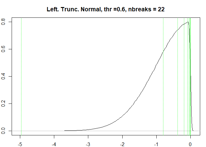
testresults <-
benchmarkdist(leftnorm, 0.6, title = "Left. Trunc. Normal")
#> [1] "prop:0.574960895030618 nhead:2873704"
#> [1] "prop:0.51244526228171 nhead:1472616"
#> [1] "prop:0.503100604638276 nhead:740874"
#> [1] "prop:0.501235027818495 nhead:371352"
#> [1] "prop:0.499935371291928 nhead:185652"
#> [1] "prop:0.499935362937108 nhead:92814"
#> [1] "prop:0.499730644083867 nhead:46382"
#> [1] "prop:0.500452761847268 nhead:23212"
#> [1] "prop:0.502240220575564 nhead:11658"
#> [1] "prop:0.490478641276377 nhead:5718"
#> [1] "prop:0.508219657222805 nhead:2906"
#> [1] "prop:0.487267721954577 nhead:1416"
#> [1] "prop:0.505649717514124 nhead:716"
#> [1] "prop:0.494413407821229 nhead:354"
#> [1] "prop:0.497175141242938 nhead:176"
#> [1] "prop:0.488636363636364 nhead:86"
#> [1] "prop:0.511627906976744 nhead:44"
#> [1] "prop:0.454545454545455 nhead:20"
#> [1] "prop:0.5 nhead:10"
#> [1] "prop:0.4 nhead:4"
#> [1] "prop:0.5 nhead:2"
#> [1] "prop:0 nhead:0"
#> [1] "Breaks found: 22 , Intervals: 23"
#> [1] -4.9605354548 -0.7984148615 -0.3786370780 -0.1871224722 -0.0935267116
#> [6] -0.0470891909 -0.0238467336 -0.0121898326 -0.0063800214 -0.0034807516
#> [11] -0.0020189035 -0.0012697479 -0.0009096890 -0.0007229499 -0.0006345192
#> [16] -0.0005898488 -0.0005691473 -0.0005569817 -0.0005515657 -0.0005488630
#> [21] -0.0005479547 -0.0005477666 -0.0005476086
#> Time difference of 0.489871 secs
testresults <-
  benchmarkdist(leftnorm, 0, title = "Left. Trunc. Normal", plot = FALSE)
#> [1] "prop:0.574960895030618 nhead:2873704"
#> [1] "Breaks found:  1 , Intervals: 2"
#> [1] -4.9605354548 -0.7984148615 -0.0005476086
#> Time difference of 0.279742 secs
testresults <-
  benchmarkdist(leftnorm, 1, title = "Left. Trunc. Normal", plot = FALSE)
#> [1] "prop:0.574960895030618 nhead:2873704"
#> [1] "prop:0.51244526228171 nhead:1472616"
#> [1] "prop:0.503100604638276 nhead:740874"
#> [1] "prop:0.501235027818495 nhead:371352"
#> [1] "prop:0.499935371291928 nhead:185652"
#> [1] "prop:0.499935362937108 nhead:92814"
#> [1] "prop:0.499730644083867 nhead:46382"
#> [1] "prop:0.500452761847268 nhead:23212"
#> [1] "prop:0.502240220575564 nhead:11658"
#> [1] "prop:0.490478641276377 nhead:5718"
#> [1] "prop:0.508219657222805 nhead:2906"
#> [1] "prop:0.487267721954577 nhead:1416"
#> [1] "prop:0.505649717514124 nhead:716"
#> [1] "prop:0.494413407821229 nhead:354"
#> [1] "prop:0.497175141242938 nhead:176"
#> [1] "prop:0.488636363636364 nhead:86"
#> [1] "prop:0.511627906976744 nhead:44"
#> [1] "prop:0.454545454545455 nhead:20"
#> [1] "prop:0.5 nhead:10"
#> [1] "prop:0.4 nhead:4"
#> [1] "prop:0.5 nhead:2"
#> [1] "prop:0 nhead:0"
#> [1] "Breaks found:  22 , Intervals: 23"
#>  [1] -4.9605354548 -0.7984148615 -0.3786370780 -0.1871224722 -0.0935267116
#>  [6] -0.0470891909 -0.0238467336 -0.0121898326 -0.0063800214 -0.0034807516
#> [11] -0.0020189035 -0.0012697479 -0.0009096890 -0.0007229499 -0.0006345192
#> [16] -0.0005898488 -0.0005691473 -0.0005569817 -0.0005515657 -0.0005488630
#> [21] -0.0005479547 -0.0005477666 -0.0005476086
#> Time difference of 0.6450229 secs

testresults <-
  benchmarkdist(leftnorm, 200, title = "Left. Trunc. Normal", plot = FALSE)
#> [1] "prop:0.574960895030618 nhead:2873704"
#> [1] "prop:0.51244526228171 nhead:1472616"
#> [1] "prop:0.503100604638276 nhead:740874"
#> [1] "prop:0.501235027818495 nhead:371352"
#> [1] "prop:0.499935371291928 nhead:185652"
#> [1] "prop:0.499935362937108 nhead:92814"
#> [1] "prop:0.499730644083867 nhead:46382"
#> [1] "prop:0.500452761847268 nhead:23212"
#> [1] "prop:0.502240220575564 nhead:11658"
#> [1] "prop:0.490478641276377 nhead:5718"
#> [1] "prop:0.508219657222805 nhead:2906"
#> [1] "prop:0.487267721954577 nhead:1416"
#> [1] "prop:0.505649717514124 nhead:716"
#> [1] "prop:0.494413407821229 nhead:354"
#> [1] "prop:0.497175141242938 nhead:176"
#> [1] "prop:0.488636363636364 nhead:86"
#> [1] "prop:0.511627906976744 nhead:44"
#> [1] "prop:0.454545454545455 nhead:20"
#> [1] "prop:0.5 nhead:10"
#> [1] "prop:0.4 nhead:4"
#> [1] "prop:0.5 nhead:2"
#> [1] "prop:0 nhead:0"
#> [1] "Breaks found:  22 , Intervals: 23"
#>  [1] -4.9605354548 -0.7984148615 -0.3786370780 -0.1871224722 -0.0935267116
#>  [6] -0.0470891909 -0.0238467336 -0.0121898326 -0.0063800214 -0.0034807516
#> [11] -0.0020189035 -0.0012697479 -0.0009096890 -0.0007229499 -0.0006345192
#> [16] -0.0005898488 -0.0005691473 -0.0005569817 -0.0005515657 -0.0005488630
#> [21] -0.0005479547 -0.0005477666 -0.0005476086
#> Time difference of 0.5481331 secs

testresults <-
  benchmarkdist(leftnorm, -100, title = "Left. Trunc. Normal", plot = FALSE)
#> [1] "prop:0.574960895030618 nhead:2873704"
#> [1] "Breaks found:  1 , Intervals: 2"
#> [1] -4.9605354548 -0.7984148615 -0.0005476086
#> Time difference of 0.3148251 secs


testresults <-
  benchmarkdist(logcauchdist, 0.7896, title = "LogCauchy", plot = FALSE)
#> [1] "prop:3.16580735701571e-05 nhead:158"
#> [1] "prop:0.20253164556962 nhead:32"
#> [1] "prop:0.34375 nhead:11"
#> [1] "prop:0.363636363636364 nhead:4"
#> [1] "prop:0.5 nhead:2"
#> [1] "prop:0.5 nhead:1"
#> [1] "Breaks found:  6 , Intervals: 7"
#> [1]  0.000000e+00 3.600688e+302 1.137365e+307 5.236743e+307 9.915649e+307
#> [6] 1.411160e+308 1.637900e+308 1.725945e+308
#> Time difference of 0.189255 secs
testresults <-
  benchmarkdist(logcauchdist, 0, title = "LogCauchy", plot = FALSE)
#> [1] "prop:3.16580735701571e-05 nhead:158"
#> [1] "Breaks found:  1 , Intervals: 2"
#> [1]  0.000000e+00 3.600688e+302 1.725945e+308
#> Time difference of 0.1979871 secs
testresults <-
  benchmarkdist(logcauchdist, 1, title = "LogCauchy", plot = FALSE)
#> [1] "prop:3.16580735701571e-05 nhead:158"
#> [1] "prop:0.20253164556962 nhead:32"
#> [1] "prop:0.34375 nhead:11"
#> [1] "prop:0.363636363636364 nhead:4"
#> [1] "prop:0.5 nhead:2"
#> [1] "prop:0.5 nhead:1"
#> [1] "Breaks found:  6 , Intervals: 7"
#> [1]  0.000000e+00 3.600688e+302 1.137365e+307 5.236743e+307 9.915649e+307
#> [6] 1.411160e+308 1.637900e+308 1.725945e+308
#> Time difference of 0.2495902 secs

# On non skewed or left tails thresold should be stressed beyond 50%,
# otherwise just the first iter (i.e. min, mean, max) is returned.
par(opar)


knitr::kable(testresults[-1, ], format = "markdown", row.names = FALSE)
| Title |
nsample |
thresold |
nbreaks |
time_secs |
| Pareto Dist |
5,000,000 |
0.4000 |
15 |
0.419203042984009 |
| Pareto Dist |
5,000,000 |
0.0000 |
2 |
0.335700988769531 |
| Pareto Dist |
5,000,000 |
1.0000 |
15 |
0.396288871765137 |
| ExpDist |
5,000,000 |
0.4000 |
16 |
0.341656923294067 |
| ExpDist |
5,000,000 |
0.0000 |
2 |
0.205184936523438 |
| ExpDist |
5,000,000 |
1.0000 |
17 |
0.422024965286255 |
| LogNorm |
5,000,000 |
0.7500 |
15 |
0.368312835693359 |
| LogNorm |
5,000,000 |
0.0000 |
2 |
0.181805849075317 |
| LogNorm |
5,000,000 |
1.0000 |
15 |
0.39214301109314 |
| Weibull |
5,000,000 |
0.2500 |
2 |
0.352260112762451 |
| Weibull |
5,000,000 |
0.0000 |
2 |
0.215781927108765 |
| Weibull |
5,000,000 |
1.0000 |
17 |
0.413298845291138 |
| Normal |
5,000,000 |
0.8000 |
17 |
0.484923839569092 |
| Normal |
5,000,000 |
0.0000 |
2 |
0.248221158981323 |
| Normal |
5,000,000 |
1.0000 |
17 |
0.433116912841797 |
| Left. Trunc. Normal |
4,998,086 |
0.6000 |
22 |
0.489871025085449 |
| Left. Trunc. Normal |
4,998,086 |
0.0000 |
2 |
0.279742002487183 |
| Left. Trunc. Normal |
4,998,086 |
1.0000 |
22 |
0.645022869110107 |
| Left. Trunc. Normal |
4,998,086 |
200.0000 |
22 |
0.548133134841919 |
| Left. Trunc. Normal |
4,998,086 |
-100.0000 |
2 |
0.314825057983398 |
| LogCauchy |
4,990,828 |
0.7896 |
7 |
0.189254999160767 |
| LogCauchy |
4,990,828 |
0.0000 |
2 |
0.197987079620361 |
| LogCauchy |
4,990,828 |
1.0000 |
7 |
0.249590158462524 |
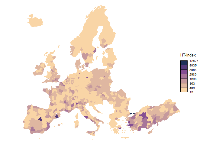
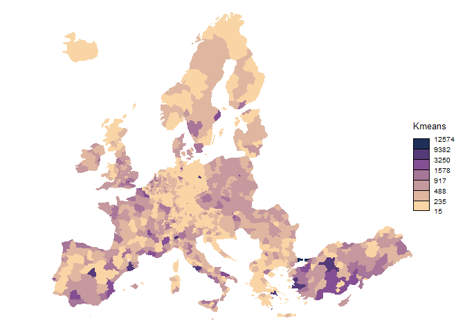
# 5. Case study: Population----
library(cartography)
library(sf)
#> Warning: package 'sf' was built under R version 3.5.3
#> Linking to GEOS 3.6.1, GDAL 2.2.3, PROJ 4.9.3
library(classInt)
#> Warning: package 'classInt' was built under R version 3.5.3

nuts3 <- st_as_sf(nuts3.spdf)
nuts3 <- merge(nuts3, nuts3.df)

nrow(nuts3)
#> [1] 1448

nuts3$var <- nuts3$pop2008 / 1000 #Thousands

opar <- par(no.readonly = TRUE)
par(mar = c(3, 2.5, 2, 1))
plot(density(nuts3$var),
     main = "NUTS3 Pop2008 (thousands)",
     ylab = "",
     xlab = "")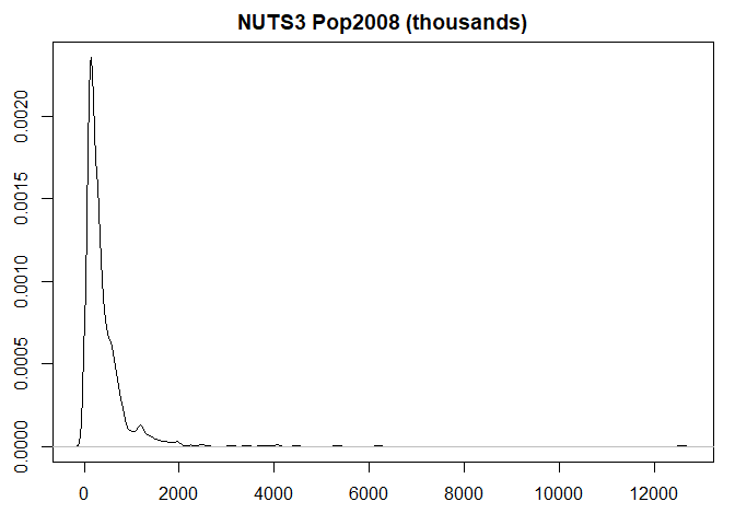
#benchmark
init <- Sys.time()
brks_ht <- ht_index(nuts3$var)
#> [1] "prop:0.31767955801105 nhead:460"
#> [1] "prop:0.267391304347826 nhead:123"
#> [1] "prop:0.252032520325203 nhead:31"
#> [1] "prop:0.32258064516129 nhead:10"
#> [1] "prop:0.3 nhead:3"
#> [1] "prop:0.333333333333333 nhead:1"
#> [1] "Breaks found:  6 , Intervals: 7"
#> [1]    15.4710   402.6459   862.5118  1638.0025  2979.9322  5084.1036  8035.3390
#> [8] 12573.8360
Sys.time() - init
#> Time difference of 0.0009970665 secs

init <- Sys.time()
brks_fisher <-
  classIntervals(nuts3$var, style = "fisher", n = 7)$brks
Sys.time() - init
#> Time difference of 0.0219841 secs

init <- Sys.time()
brks_kmeans <-
  classIntervals(nuts3$var, style = "kmeans", n = 7)$brks
Sys.time() - init
#> Time difference of 0.007397175 secs


cols <- c(carto.pal("harmo.pal", 7))


par(mar = c(0, 0, 0, 0))
choroLayer(
  nuts3,
  var = "var",
  breaks = brks_ht,
  legend.title.txt = "HT-index",
  col = cols,
  border = NA,
  legend.pos = "right"
)
choroLayer(
  nuts3,
  var = "var",
  breaks = brks_fisher,
  legend.title.txt = "Fisher",
  col = cols,
  border = NA,
  legend.pos = "right"
)

choroLayer(
  nuts3,
  var = "var",
  breaks = brks_kmeans,
  legend.title.txt = "Kmeans",
  col = cols,
  border = NA,
  legend.pos = "right"
)
par(opar)

paste0("Full running time:", Sys.time() - initrun)
#> [1] "Full running time:24.792090177536"
Created on 2020-03-15 by the reprex package (v0.3.0)


