Geopandas scatterplot jenks colors to pydeck deck.gl (ScatterplotLayer & GeoJsonLayer)

pydeck.py

import geopandas as gpd
import pydeck as pdk

gdf = gpd.read_parquet("points.parquet") # lat lon columns in EPSG:4326 included
polys = gpd.read_parquet("polys.parquet") # load polygons/multipolygons
polys['geometry'] = polys['geometry'].buffer(0) # a trick in geopandas to fix invalid geometries, holes etc.
polys = polys.to_crs("4326") # IMPORTANT: Must be in 4326, else map won't display

def hex_to_rgb(hex_color):
    hex_color = hex_color.lstrip('#')
    return tuple(int(hex_color[i:i+2], 16) for i in (0, 2, 4))
color_mapping = {
        1: '#006837',  # dark green
        2: '#86cb66',  # green
        3: '#ffffbf',  # yellow
        4: '#f98e52',  # orange
        5: '#a50026'   # dark red
    }
gdf['rgb_color'] = gdf['naturalbreaks'].map(color_mapping).apply(hex_to_rgb)

reduced_gdf = gdf#.iloc[:10000] # reduce rows for tests

view = pdk.data_utils.compute_view(reduced_gdf[["lon", "lat"]])

#Red: (255, 0, 0)
#Blue: (0, 0, 255)
#Green: (0, 255, 0)
#Yellow: (255, 255, 0)

# custom colors: https://deckgl.readthedocs.io/en/latest/gallery/polygon_layer.html?highlight=get_fill_color
all_points = pdk.Layer(
    'ScatterplotLayer',   
    reduced_gdf,
    get_position=['lon', 'lat'],
    auto_highlight=True,
    get_radius=30,          
    opacity=0.9,
    get_fill_color="rgb_color",
    pickable=True)

improvement_points = pdk.Layer(
    'ScatterplotLayer',    
    gdf[gdf["rank_improved"] == True],
    get_position=['lon', 'lat'],
    auto_highlight=True,
    get_radius=100,          # Radius is given in meters
    opacity=0.1,
    get_fill_color=[0, 0, 255], 
    pickable=True)

desert_points = pdk.Layer(
    'ScatterplotLayer',     # Change the `type` positional argument here
    gdf[gdf["rank_improved"] == False], # only the 64 moved points
    get_position=['lon', 'lat'],
    auto_highlight=True,
    get_radius=100,          # Radius is given in meters
    opacity=0.1,
    get_fill_color=[255,0, 0],
    pickable=True)

polygon = pdk.Layer(
    'GeoJsonLayer',
    data=polys,
    get_fill_color=[255, 255, 255], 
    opacity=0.3,
    get_line_color=[0,0,0],
    filled=True,
    stroked=True,
    line_width_min_pixels=0.5,
    pickable=True
)

r = pdk.Deck([polygon,improvement_points,desert_points,all_points],
          #map_provider=None, # if no basemap needed
          initial_view_state=view)

r.to_html("test.html", notebook_display=True,iframe_height=800) # set iframe for jupyter, else remove.
# As of 16/11/2023 No method for just displaying without saving and setting height available

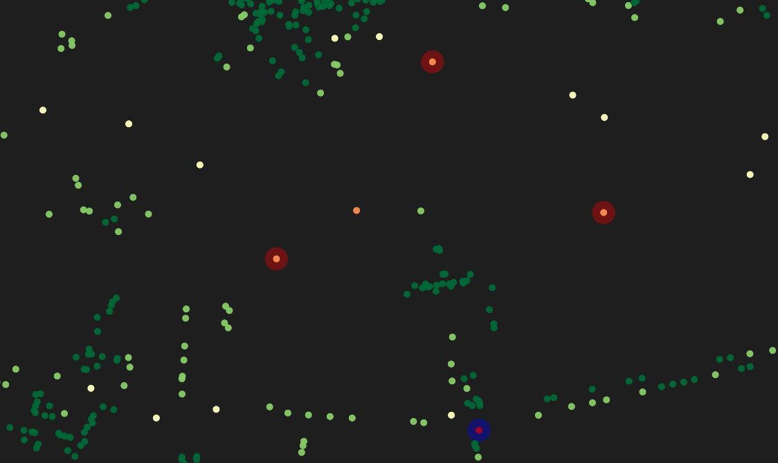
Result looks like this (displayed without Polygons here) and is very performant. Tested with 55.000 points in Firefox - works very well without any lag on mediocre laptop hardware (unlike Folium/Leaflet where I tested the exact same). The html file size depends heavily on the amount of columns you want to display. In my case with ~20 columns the file size varied between 50-80 Mb. Gzipped it becomes 3-5 Mb - perfect for quickly sending to coworkers.