|
#!/usr/bin/env python |
|
# -*- coding: utf-8 -*- |
|
""" |
|
Translated from a MATLAB script (which also includes C-weighting, octave |
|
and one-third-octave digital filters). |
|
|
|
Author: Christophe Couvreur, Faculte Polytechnique de Mons (Belgium) |
|
[email protected] |
|
Last modification: Aug. 20, 1997, 10:00am. |
|
BSD license |
|
|
|
http://www.mathworks.com/matlabcentral/fileexchange/69 |
|
Translated from adsgn.m to Python 2009-07-14 [email protected] |
|
""" |
|
|
|
from numpy import pi, polymul |
|
from scipy.signal import bilinear |
|
|
|
|
|
def A_weighting(fs): |
|
"""Design of an A-weighting filter. |
|
|
|
b, a = A_weighting(fs) designs a digital A-weighting filter for |
|
sampling frequency `fs`. Usage: y = scipy.signal.lfilter(b, a, x). |
|
Warning: `fs` should normally be higher than 20 kHz. For example, |
|
fs = 48000 yields a class 1-compliant filter. |
|
|
|
References: |
|
[1] IEC/CD 1672: Electroacoustics-Sound Level Meters, Nov. 1996. |
|
|
|
""" |
|
# Definition of analog A-weighting filter according to IEC/CD 1672. |
|
f1 = 20.598997 |
|
f2 = 107.65265 |
|
f3 = 737.86223 |
|
f4 = 12194.217 |
|
A1000 = 1.9997 |
|
|
|
NUMs = [(2*pi * f4)**2 * (10**(A1000/20)), 0, 0, 0, 0] |
|
DENs = polymul([1, 4*pi * f4, (2*pi * f4)**2], |
|
[1, 4*pi * f1, (2*pi * f1)**2]) |
|
DENs = polymul(polymul(DENs, [1, 2*pi * f3]), |
|
[1, 2*pi * f2]) |
|
|
|
# Use the bilinear transformation to get the digital filter. |
|
# (Octave, MATLAB, and PyLab disagree about Fs vs 1/Fs) |
|
return bilinear(NUMs, DENs, fs) |


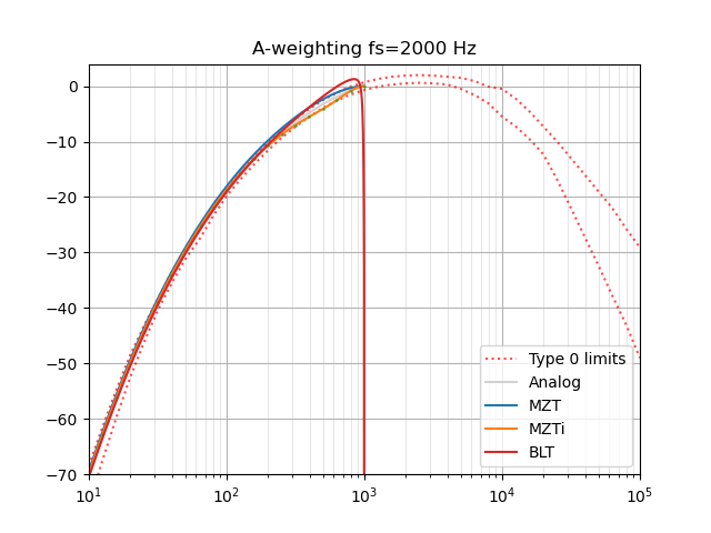

So I'm looking at my "improved" version from 2018, which is based on the MZTi method and it does indeed have better frequency response at high frequencies:
But I think the reason I didn't push it was because I wasn't sure I was doing it right. "Since the mapping wraps the s-plane's jω axis around the z-plane's unit circle repeatedly, any zeros (or poles) greater than the Nyquist frequency will be mapped to an aliased location." And I'm not sure if those need to be removed first, depending on the sampling rate, etc. At lower sample rates it gets worse, so it still needs some work. (Also the aliased Nyquist tail could be pushed down a bit to improve the overall average accuracy.)
This paper just describes the same BLT solution as this gist, and has a table of the minimum required sample rate to meet the tolerances:
There are probably other papers that describe better methods, I should look for them.