R | ECharts | boxplot

boxplot.R

library(echarty); library(dplyr)

# 1) boxplot with calculation in R ---------------------

p <- ec.init()
p$x$opts$series <- list(
	list(type='boxplot', name='mpg', data=list(boxplot.stats(mtcars$mpg)$stats)), 
	list(type='boxplot', name='hp',  data=list(boxplot.stats(mtcars$hp)$stats)), 
	list(type='boxplot', name='disp',data=list(boxplot.stats(mtcars$disp)$stats))
)	
p$x$opts$xAxis <- list(name='item', type = 'category')
p$x$opts$legend <- list(ii='')
p


# 2) boxplot calculation in ECharts ---------------------
#    source: https://echarts.apache.org/examples/en/editor.html?c=boxplot-multi

grps <- list()     # data is 3 groups of 18 experiments
for (grp in 1:3) {
	seriesData <- list()
	for (i in 1:18) {
		cate <- runif(10, 1, 200)
		seriesData <- append(seriesData, list(cate))
	}
	grps[[grp]] <- seriesData
}

p <- ec.init()
p$x$opts$dataset <- list(
  list(source=grps[[1]]), list(source=grps[[2]]), list(source=grps[[3]]),
	list(fromDatasetIndex=0, transform=list(type='boxplot', config=list(itemNameFormatter='expr {value}'))),
	list(fromDatasetIndex=1, transform=list(type='boxplot', config=list(itemNameFormatter='expr {value}'))),
	list(fromDatasetIndex=2, transform=list(type='boxplot', config=list(itemNameFormatter='expr {value}')))
)
p$x$opts$series[[1]] <- list(type = 'boxplot', datasetIndex=3, name='c1')
p$x$opts$series[[2]] <- list(type = 'boxplot', datasetIndex=4, name='c2')
p$x$opts$series[[3]] <- list(type = 'boxplot', datasetIndex=5, name='c3')
p$x$opts$xAxis <- list(type = 'category')
p$x$opts$legend <- list(ii='')
p


# 3) horizontal boxplot with outliers ---------------------
#    source: https://echarts.apache.org/examples/en/editor.html?c=boxplot-light-velocity2
# with ECharts boxplot calculations:
# lower whisker = Q1 - 1.5 * IQR
# upper whisker = Q3 + 1.5 * IQR

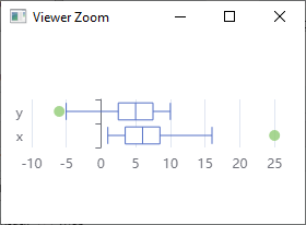
df <- data.frame(x = c(1:10, 25), y = c(1:10, -6))

p <- ec.init()
p$x$opts$dataset <- list(list(source= ec.data(data.frame(t(df)), header=FALSE)),
                         list(transform= list(type='boxplot')),
                         list(fromDatasetIndex= 1, fromTransformResult= 1))
p$x$opts$yAxis <- list(type= 'category', boundaryGap= TRUE,
                       axisLabel= list(formatter=htmlwidgets::JS("function(i){ return ['x','y'][i]; }")))
p$x$opts$series <- list(
  list(name= 'boxplot', type= 'boxplot', datasetIndex= 1),
  list(name= 'outlier', type= 'scatter', encode= list( x= 1, y= 0), datasetIndex= 2)
)
p

idea from @rleyvasal

horizontal boxplots with outliers, data from @Laurent-Smeets-GSS-Account

Grouped box plot with multiple variables - inquiry by @guybrettrobertson
Aah, ggplot2 to haunt us again ! A mighty one-liner indeed.
ggplot(data, aes(x=variety, y=note, fill=treatment)) + geom_boxplot()
Here is how to replicate with echarty and the native ECharts boxplot utilities. See more boxplots in the Gallery.

# data/concept from https://www.r-graph-gallery.com/265-grouped-boxplot-with-ggplot2.html
variety = rep(LETTERS[1:7], each=40)
treatment = rep(c("high","low"),each=20)
note = seq(1:280)+sample(1:150, 280, replace=T)
d <- data.frame(variety, treatment ,  note)

# --------- prep raw data for ECharts
library(dplyr)
series <- list()
df <- d |> group_by(treatment) |> group_split()
dataset <- lapply(df, function(dd) { 
	dv <- dd |> group_by(variety) |> group_split()
	list(source= lapply(dv, function(vv) vv$note) )
})
for (i in 1:length(df)) { 
	dataset <- append(dataset, list(list(
		fromDatasetIndex= i-1, transform= list(type= 'boxplot')))) 
	series <- append(series, list(list(
		name= df[[i]]$treatment[1], 
		type= 'boxplot', datasetIndex= i+length(df)-1)) )
}
xax <- paste(unique(d$variety), collapse="','")   # X-axis labels
xax <- paste0("(v) => { return ['",xax,"'][v]; }")

# ----------- visualization
library(echarty)
p <- ec.init()
p$x$opts$xAxis <- list(type= 'category', axisLabel= list(formatter= htmlwidgets::JS(xax)))
p$x$opts$dataset <- dataset
p$x$opts$series <- series
p$x$opts$legend <- list(show=TRUE)
p

Note: if you like this solution, please consider granting a Github star ⭐ to echarty.

Now data prep code has been merged into echarty. Use ec.data(format='boxplot') to submit your data, then fill dataset and series attributes.
The only requirement is for column position. Details in help ?ec.data. Thanks to @guybrettrobertson for initiating this enhancement.

variety = rep(LETTERS[1:7], each=40)
note = seq(1:280)+sample(1:150, 280, replace=T)
treatment = rep(c("high","low"),each=20)
d <- data.frame(treatment, note, variety)

library(echarty)
#  another example:
# ds <- mtcars |> relocate(am,mpg) |> group_by(cyl) |> ec.data(format='boxplot')

ds <- d |> group_by(variety) |> ec.data(format='boxplot')
p <- ec.init()
p$x$opts <- list(
	xAxis= list(type= 'category'),  
	yAxis= list(show= TRUE),
	dataset= ds$dataset, 
	series= ds$series, 
	legend= list(show= TRUE)
)
p

Note: if you like this solution, please consider granting a Github star ⭐ to echarty.