I’m currently working on an OCR project with some of my Vision researcher/engineer colleagues: FVI. The job is to extract pieces of information from a Vietnamese ID card.
In research progress, I wandered the internet and found some useful articles (e.g. Dropbox, Zocdoc, Facebook) about how to build an OCR system. But none of this explained clearly to me a complete intuition how to bring these research models into a production environment. So our team had a hard time (roughly 6 months) struggling to build an accurate, production-ready and scalable OCR system.
And in this post, I want to share with you our experience (research, architecture, and deploy process) in hope to clear the mist of building and deploying a complete Deep Learning project in general, and OCR task in particular.
Our structure consists of 3 basic components: Cropper, Detector, Reader. Each component has its own model and train/validation/test process. So it can be easy to plug and play plugins to improve the system, better than a black box of a single end-to-end model.

This component locates 4 corners of the ID card and then crop its quadrangular shape. The meaning of this is to make easier for word detection tasks (e.g. reduce noises and variances) which comes after.
Since the common object detection model only returns 2 corners (a rectangular box), we use a little trick by treating each corner as an object with its own unique class and then detect 4 corners. The geometric transformation after locating 4 corners is trivial.

Our detection model we are using is single shot detector: SSD ( SSD: Single Shot MultiBox Detector), with feature extractor is MobileNet v2 (MobileNetV2: Inverted Residuals and Linear Bottlenecks).
SSD provides us fast inference speed, while MobileNet v2 decreases the number of operations and memory but still preserves good accuracy.
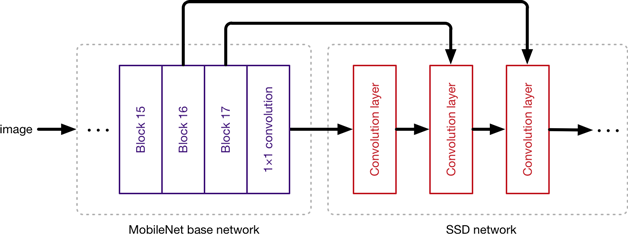
Image courtesy of Matthijs Hollemans, source
This component extracts rectangular shapes contain word tokens belongs to each class (e.g. ID number, name, address, date of birth). We sort them depends on coordinates and then parse them to the Reader.
We also utilizes SSD for this task just like the Cropper, but with different feature extractor: Resnet FPN (Deep Residual Learning for Image Recognition, Feature Pyramid Networks for Object Detection)
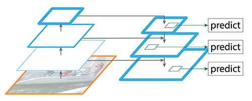
Image in the FPN paper, and courtesy of Jonathan Hui, source
Resnet FPN assures us state-of-the-art accuracy, and supports multi-scale of an image so the model can deal with various input situations.
Given some words and their orders for each region class, we do batch inferencing to the Reader model to get the string results.
The model architecture we use is a word-level reader, utilizes the Google's Attention OCR architecture ( Attention-based Extraction of Structured Information from Street View Imagery) with some little tweaks.

Image in Attention OCR paper
First, we use 1 view instead of 4 views for each word image because the text detected is mostly vertical after the Cropper phase.
And then use the same Inception Resnet v2 layer
(Inception-v4, Inception-ResNet and the Impact of Residual Connections on Learning) cut at Mixed_6a for feature extraction,
followed by LSTM layer and then attention decoder.
For gradient descent optimization, we use Adadelta with initial learning rate 1.0 rather than stochastic gradient descent (SGD) with momentum described in the paper. Mainly reason is Adadelta adapts the learning rate to the parameters, thus no troubling tuning the learning rate in train process.
This Reader model achieves more than 99% for character accuracy and often with 1-2% decreases in word accuracy. The combined end-to-end system (Cropper -> Detector -> Reader) achieves approximately 90% accuracy for each region class.
Theoretically, we can do better with some strategy like synthetic data, curriculum training, and so much more. But with the first public version we think this is enough and decide to give it a go in the production, and then update follow client feedbacks.
Here a diagram of our structure used in a real-life scenario.

The problem is how to bring these components into the production environment.
The naive way is to pre-load the trained checkpoints and write some additional query function to infer the model. But it's not an optimized way. It eats resources with bloated memory, has high latency queries and high risk of CPU spikes.
A better way is to freeze to model first (called a Frozen Graph, tutorial like this) to clear the mentioned problem.
But we want a more mature way of serving the trained models, say low-latency high-throughput requests, zero-downtime model update, batch inferencing request, consistent API for inferencing. Luckily, Google has a solution for us, enter Tensorflow Serving.
Tensorflow Serving uses SavedModel with version tag. For example, here I have a 1-version Cropper, 1-version Detector, and 2-version Reader.
Cropper/
  1/

Detector/
  1/

Reader/
  1/
  2/
    saved_model.pb
    variables/
      variables.index
And you can load all of these models into Tensorflow Serving at once (YES, multiple models serving) by specifying a model base path config (for example, serving.config):
model_config_list: {
  config: {
      name: "cropper",
      base_path: "/absolute/path/to/cropper",
      model_platform: "tensorflow"
  },
  config: {
      name: "detector",
      base_path: "/absolute/path/to/detector",
      model_platform: "tensorflow"
  },
  config: {
      name: "reader",
      base_path: "/absolute/path/to/reader",
      model_platform: "tensorflow"
  }
}
and boot up Tensorflow Serving with appropriate flag:
tensorflow_model_server --model_config_file=/absolute/path/to/serving.configThe trouble way is you have to export model with trained weights to SavedModel format first.

A sample script to export I provide here. The trick is you make use of Tensorflow Saver.
Specifically, SavedModel wraps a TensorFlow Saver. The Saver is primarily used to generate the variable checkpoints. source
And the second important thing is you understand what input and output node your model is having.
# ...

with tf.Session() as sess:
    tf.train.Saver().restore(sess, FLAGS.checkpoint)

    # images_placeholder as input node
    inputs = {'input': tf.saved_model.utils.build_tensor_info(INPUT_PLACEHOLDER)}

    # get output node through node name
    out_classes = sess.graph.get_tensor_by_name('YOUR_OUTPUT_NODE_NAME')
    outputs = {'output':  tf.saved_model.utils.build_tensor_info(out_classes)}

    signature = tf.saved_model.signature_def_utils.build_signature_def(
        inputs=inputs,
        outputs=outputs,
        method_name=tf.saved_model.signature_constants.PREDICT_METHOD_NAME)

    legacy_init_op = tf.group(tf.tables_initializer(), name='legacy_init_op')

    # Save out the SavedModel
    builder = tf.saved_model.builder.SavedModelBuilder(FLAGS.saved_dir)
    builder.add_meta_graph_and_variables(
        sess, [tf.saved_model.tag_constants.SERVING],
        signature_def_map={
            tf.saved_model.signature_constants.
            DEFAULT_SERVING_SIGNATURE_DEF_KEY:
            signature
        },
        legacy_init_op=legacy_init_op)
builder.save()Now is the full look of our backend service:

There are 2 small services (components) we mainly take care of: api and serving.
serving is Tensorflow Serving as we mentioned, and api (which provides RESTful API for clients) connects with serving through grpc.
Luckily (also), we don't have to take care much of Protocol Buffers logics and just make use of tensorflow-serving-api library.
A sample use I provide:
import tensorflow as tf
from tensorflow_serving.apis import predict_pb2
from tensorflow_serving.apis.prediction_service_pb2_grpc import PredictionServiceStub

import grpc
import cv2


# Your config
SERVICE_HOST = 'localhost:8500' # sample
MODEL_NAME = 'reader'
INPUT_SIGNATURE_KEY = 'input'
OUTPUT_SIGNATURE_KEY = 'output'

#######

# Connect to server
channel = grpc.insecure_channel(SERVICE_HOST)
stub = PredictionServiceStub(channel)

# Prepare request object
request = predict_pb2.PredictRequest()
request.model_spec.name = MODEL_NAME
request.model_spec.signature_name = tf.saved_model.signature_constants.DEFAULT_SERVING_SIGNATURE_DEF_KEY

# Copy image into request's content
img = cv2.imread('/path/to/image')
input_tensor = np.expand_dims(img, axis=0) # we do batch inferencing, so input is a 4-D tensor
request.inputs[INPUT_SIGNATURE_KEY].CopyFrom(
    tf.contrib.util.make_tensor_proto(input_tensor))

# Do inference
result = stub.Predict.future(request, 5) # 5s timeout

# Get output depends on our input/output signature, and their types
# for example, our output signature key is 'output' and has string value
word = result.result().outputs[OUTPUT_SIGNATURE_KEY].string_val[0] # we have batch result, so just take first index
Deployment is an important part, but usually a myth among Deep Learning articles.
Tensorflow Serving guide demos deploy in Kubernetes with built container images.
But we found it over-complicated and decided to use Docker Compose for simply running two pre-built images api and serving.
We have two types of deploy machines, only CPU platform, and with GPU platform.
Only CPU machine goes with common docker-compose.yml, with Dockerfile for api, and Dockerfile.serving for serving which is based from tensorflow/serving:latest-devel image.

On the other hand, GPU machine goes with custom nvidia-docker-compose.yml (which requires nvidia-docker), same Dockerfile for api, and Dockerfile.serving.gpu for serving (which is based from tensorflow:latest-devel-gpu).

One main note for running Docker Compose with GPU is inside nvidia-docker-compose.yml you have to specify runtime: nvidia.
A troublesome problem is Docker Compose default uses all GPUs so you have to set NVIDIA_VISIBLE_DEVICES environment variable to your dedicated running GPUs.
A trick I use for consistent use between Tensorflow (CUDA_VISIBLE_DEVICES) and Docker Compose is:
# nvidia-docker-compose.yml

version: '2.3'
services:
  serving:
    runtime: nvidia
    environment:
      NVIDIA_VISIBLE_DEVICES: ${CUDA_VISIBLE_DEVICES:-all}
    [...]
  [...]
By doing that, if you set CUDA_VISIBLE_DEVICES you use what GPUs you want to use. Otherwise it uses all GPUs by default.
I shared you our research, architecture, and deployment of a complete OCR system. It uses the state-of-the-art deep learning OCR model (Attention OCR), scalable with Tensorflow Serving, and ready for production deployment with the help of Docker Compose.
By using Tensorflow we have an entire ecosystem backed by Google, a typical benefit is Tensorflow Serving (which belongs to TFX). A huge support is from the community for model implementation, too.