An accelerating object in the frame of another accelerating object (special relativity)

StarshipPursuit.tex

\documentclass[crop=true, border=10pt]{standalone}
\usepackage{comment}
\begin{comment} 
:Title: Intercepting an accelerating starship
:Slug: Accelerating starship
:Tags:  special relativity
:Author: J A Miller, UAH Physics & Astronomy, [email protected], 2020/06/29

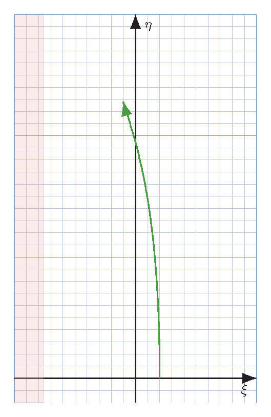
Worldline of an accelerating ship in the frame ($\xi$ - $\eta$) of another accelerating ship.

Basic plot style and colors from:
    https://gist.github.com/mcnees/45b9f53ad371c38ba6f3759df5880fb1

---------------------------------------------------------------------
Background
---------------------------------------------------------------------

The equations of motion for an object undergoing uniform proper acceleration $\alpha$ are
\begin{equation}
    \begin{split}
		x &= \frac{1}{\alpha} \cosh(\alpha \tau) - \frac{1}{\alpha} + x_0 \\
		t &= \frac{1}{\alpha} \sinh(\alpha \tau),
    \end{split}
\end{equation}
where $\tau$ is the proper time, and $x_0$ is the starting location.

Accelerated coordinates can be defined by
\begin{equation}
    \begin{split}
		\xi &= \qty[ \qty( x - x_0 + \frac{1}{\alpha} )^2 - t^2  ]^{1/2} - \frac{1}{\alpha} \\
		\eta &= \frac{1}{\alpha} \tanh^{-1} \frac{t}{x - x_0 + 1/\alpha}.
    \end{split}
\end{equation}

We can plot the motion of an accelerated object (Ship 2) in the frame of another accelerating object (Ship 1) by substituting the first set of equations into the second. In the second set, $\alpha$ and $x_0$ are for Ship 2. In the first set, $\alpha$ and $x_0$ are for Ship 1.

\end{comment}



\usepackage{tikz}
\usetikzlibrary{arrows.meta}

\usepackage{pgfplots}
\pgfplotsset{compat=1.16}

\usepackage{xcolor}
\definecolor{plum}{rgb}{0.36078, 0.20784, 0.4}
\definecolor{chameleon}{rgb}{0.30588, 0.60392, 0.023529}
\definecolor{cornflower}{rgb}{0.12549, 0.29020, 0.52941}
\definecolor{scarlet}{rgb}{0.8, 0, 0}
\definecolor{brick}{rgb}{0.64314, 0, 0}
\definecolor{sunrise}{rgb}{0.80784, 0.36078, 0}
\definecolor{lightblue}{rgb}{0.15,0.35,0.75}


% ----------------------- user specifications ------------------------

% proper acceleration of Ship 1
\newcommand*{\accel}{1.32}
% proper acceleration of Ship 2
\newcommand*{\accela}{1.0}

% maximum proper time on Ship 2
\newcommand*{\taumax}{2.6}

% calculate the inverse of accelerations
\pgfmathsetmacro{\accelinv}{1/\accel}
\pgfmathsetmacro{\accelainv}{1/\accela}

% initial starting point for Ship 1
\newcommand*{\xinit}{0}  % this is $x_0$
% initial starting point for Ship 2
\newcommand*{\xinita}{0.2}  % this is $x_0$

% define the arctanh
\pgfkeys{/pgf/declare function={arctanh(\x) = 0.5*(ln(1+\x)-ln(1-\x));}}

% inertial frame trajectory of Ship 2 as a function of its proper time
\pgfkeys{/pgf/declare function={xa(\tau) = \accelainv*(cosh(\accela*\tau)-1)+\xinita;}}
\pgfkeys{/pgf/declare function={ta(\tau) = \accelainv*sinh(\accela*\tau);}}

% define the accelerated coordinates for Ship 1 (the chase ship)
\pgfkeys{/pgf/declare function={xi(\tau) = sqrt((xa(\tau)-\xinit+\accelinv)^2 - ta(\tau)^2) - \accelinv;}}
\pgfkeys{/pgf/declare function={eta(\tau) = \accelinv*arctanh(ta(\tau)/(xa(\tau)-\xinit+\accelinv));}}

% graph boundaries
\newcommand*{\xa}{-1}  % lower left corner
\newcommand*{\ya}{-0.2}
\newcommand*{\xb}{1}  % upper right corner
\newcommand*{\yb}{3}


% ------------------------ begin figure ------------------------------

\begin{document}

\begin{tikzpicture}[
	scale=1,
	x=3cm,y=3cm,
	axisarrow/.style=-{Latex[inset=0pt,length=10pt]},
	minor gridlines/.style={cornflower!30,step=0.1,thin},
	major gridlines/.style={cornflower!60,step=1.0,thin},
	axes/.style={black,thick,axisarrow},
    ]
	
  % Draw the background grid.
	\draw [minor gridlines] (\xa,\ya) grid (\xb,\yb);
	\draw [major gridlines] (\xa,\ya) grid (\xb,\yb);

	% Clip everything that falls outside the grid
	\clip(\xa,\ya) rectangle (\xb,\yb);
	
	% Draw Axes
	\draw[axes] (0,\ya) -- (0,\yb);
	\node[right,inner sep=0pt] at (0.07,2.9) {$\eta$};
	\draw[axes] (\xa,0) -- (\xb,0);
	\node[inner sep=0pt] at (0.9,-0.1) {$\xi$};
	
	% Event horizon
    \draw[fill=scarlet!40,opacity=0.2] (\xa,\ya)--(-\accelinv,\ya)--(-\accelinv,\yb)--(\xa,\yb)--(\xa,\ya);	
	
	% Draw the worldline of the alien	
	\draw[domain=0:\taumax,smooth,variable=\tau,chameleon,thick,samples=500,axisarrow] 
             plot ({xi(\tau)},{eta(\tau)});
	
	% Some more labels	
	%\node[right,inner sep=0pt] at (4,1.4) {Worldline};
	%\node[above right,inner sep=0pt] at (6,4) {$\alpha = 1, x_0 = 0$};

	
\end{tikzpicture}
			

\end{document}

Example output, using the parameters above.