Linear Algebra (and some calculus (and some geometric algebra))

geoalg.md

Better version

Sources

Geometric Algebra

The geometric product

We define the geometric product of two vector $u$ and $v$ as:

$$ uv=u\cdot v+u\wedge v $$

The dot product

$u\cdot v$ is the classic dot product. A few reminders about the dot product:

• $u\cdot v= \begin{bmatrix}a && b\end{bmatrix} \cdot \begin{bmatrix} c \\ d\end{bmatrix} = ac+bd $
• the dot product is a scalar
• geometrically, it is the factor which shall be apply to a unit vector to obtain the projection of the other vector onto the former
• the dot product is commutative: $u\cdot v = v\cdot u$
• the dot product of two perpendicular vectors is 0 ($1 \times 0 + 0 \times 1 = 0)$
• $u\cdot v= \left\lVert u \right\rVert\left\lVert v \right\rVert \cos\theta$ if $u$ and $v$ form the angle $\theta$

The wedge (or exterior) product

$u\wedge v$ is the wedge product. It can also be called the exterior product and shall be confused with the outer product.

The wedge product represent the are of the parallelogram formed by the two vector. For example, $i\wedge j = 1$ because the parallelogram (square) of the orthogonal basis $\{ i, j \}$ is a square of area 1.

The wedge product is not communitative. It is positive when the the angle formed by $u$ and $v$ is positive (going counterclockwise). However, if $u\wedge v$ is positive then $v\wedge u$. In fact, as the paralelogram formed is still very much the same, we can write:

$$ u\wedge v = -u\wedge v $$

When $u$ and $v$ are parallels, $u\wedge v=0$.

The area of the parallelogram is computed by the determinant:

$$ \begin{aligned} u\wedge v &= det(\begin{bmatrix}u && v\end{bmatrix}) \cdot i\wedge j \\\ &= \begin{vmatrix} a && c \\\ b && d \end{vmatrix} \cdot i\wedge j \\\ &=(ad-bc) \cdot i\wedge j \end{aligned} $$

Finally, using the trigonometric circle and the formula to compute the area of parallelogram, we can prove that:

$$ u\wedge v=\left\lVert u \right\rVert\left\lVert v \right\rVert \sin\theta \cdot i\wedge j $$

$u\wedge v$ is a bivector. A scalar is a 0-order quantity. A vector is a 1-order quantity. A bivector is a 2-order entity.

Back to the geometric product

As a consequence of the above, we can deduce that:

• $uu = u\cdot u + u\wedge u = \left\lVert u \right\rVert^2 + 0 = \left\lVert u \right\rVert^2$
• $uv = u\cdot v + u\wedge v = v\cdot u - v\wedge u = -vu$
• $ii = i\cdot i + i\wedge i = 1 + 0 = 1$
• $ij = i\cdot j + i\wedge j = 0 + 1 = 1$
• $(ij)^2=ijij=-ijji=-i\cdot 1 \cdot i=-ii=-1$

This last point should remind us of the imaginary number $i^2=-1$. We will note $ij=I$ so that $I^2 = -1$.

Inversion

Some operators have a way to revert their effect. Addition has subtraction. In other words, if you add the inverse of an operand, the overall effect is nill:

$$ a + 1 + (-1) = x $$

In the case scalar multiplication:

$$ a \times x \times \frac{1}{x} = a $$

there is even a notation for it: $\frac{1}{x} = x^{-1}$. This inverse is such as:

$$ x \times x^{-1} = 1 $$

The geometric product can also revert its effect by applying an invert vector:

$$ \begin{aligned} uu &= u^2=u\cdot u=\left\lVert u \right\rVert^2 \\\ u^2 &= \left\lVert u \right\rVert^2 \\\ \frac{u^2}{\left\lVert u \right\rVert^2}&=1 \\\ \underbrace{\frac{u}{\left\lVert u \right\rVert^2}}_{=u^{-1}}u &= 1 \\\ u^{-1} &= \frac{u}{\left\lVert u \right\rVert^2} \end{aligned} $$

The condition, of course, is $u \neq 0$.

Special cases

Due to the specificities of the dot and wedge product, when vectors are parallel, the geometric product commutes:

$$ uv = u\cdot v + \underbrace{u\wedge v}_{=0} = u\cdot v = vu $$

When perpendicular, it is the other way around, it anticommutes:

$$ uv = \underbrace{u\cdot v}_{=0} + u\wedge v = u\wedge v = -vu $$

Interesting identities

$$ \begin{aligned} uv &= u\cdot v + u\wedge v \\\ vu &= v\cdot u + v\wedge u = v\cdot u - u\wedge v \\\ uv + vu &= 2u\cdot v \\\ u\cdot v&=\frac{1}{2}(uv + vu) \end{aligned} $$

By analogy:

$$ \begin{aligned} uv-vu &= 2u\wedge v \\\ u\wedge v &= \frac{1}{2}(uv-vu) \\\ \end{aligned} $$

Projection

From these two identifies, an interesting formula can be devised. Let's calculate the projection of $u$ on $v$. $u_{\|}$ is the projection $v$ of $u$ and is parallel to v. $u_{\perp}$ is vector that goes from $u_{\|}$ to $u$ such that:

$$ u = u_{\|} + u_{\perp} $$

Let's see how to express a projection using the geometric product:

$$ \begin{aligned} uv &= u_{\|}v + u_{\perp}v \\\ uv &= u_{\|}v - vu_{\perp} \\\ uv &= u_{\|}v - v(u - u_{\|}) = u_{\|}v - vu + vu_{\|} \\\ uv &= u_{\|}v - vu + u_{\|}v \\\ uv + vu &= 2u_{\|}v \\\ u_{\|}v &= \underbrace{\frac{1}{2}(uv + vu)}_{u\cdot v} \\\ u_{\|} &= (u\cdot v)v^{-1} \end{aligned} $$

Note that, as a special case, if $v$ is a unit vector, then $\frac{v}{\|v\|^2} = 1$ then $v=v^{-1}$

$$ u_{\|} = (u\cdot v)v $$

Now for the wedge product:

$$ \begin{aligned} u &= u_{\|} + u_{\perp} \\\ u_{\perp} &= u - u_{\|} \\\ u_{\perp} &= u - (u\cdot v)v^{-1} \\\ u_{\perp} &= (uv - u\cdot v)v^{-1} \\\ u_{\perp} &= (u\wedge v)v^{-1} \\\ \end{aligned} $$

Multiplying by a bivector is to rotate $v^{-1}$ (See Rotations chapter). So $u_{\perp}$ is $v^{-1}$ rotated by the bivector $u\wedge v$ and scaled by the magnitude of $u\wedge v$.

So $u_{\|}$ can be expressed by the dot product and $u_{\perp}$ can be expressed by the wedge product.

Reflections

Let's keep the mental image of the previous chapter: a vector $u$ projected onto a vector $v$ with the projection called $u_{\|}$ and parallel to $v$ and $u_{\perp}$ the rejected vector perpendicular to $v$ and going from the tip of $u_{\|}$ to the tip of $u$.

Then:

$$ u = u_{\|} + u_{\perp} $$

Now the reflection of $u$ on $v$, $u^\prime$ is simply given by

$$ u^\prime = u_{\|} - u_{\perp} $$

So:

$$ \begin{aligned} vu^\prime &= vu_{\|} - vu_{\perp} \\\ vu^\prime &= u_{\|}v + u_{\perp}v \\\ vu^\prime &= (u_{\|} + u_{\perp})v \\\ vu^\prime &= uv \end{aligned} $$

Which gives

$$ u^\prime = v^{-1}uv $$

If $v$ is a unit vector, then $v^{-1} = v$, then a reflection by this vector gives:

$$ u^\prime = vuv $$

Rotations

When dealing with vector as complex number, multiplying by $i$ would rotate the vector:

$$ (a + bi)i = ai + bi^2 = ai-b $$

Rotating the vector $\begin{bmatrix}a \\ b\end{bmatrix}$ into $\begin{bmatrix}-b \\ a\end{bmatrix}$, so a rotation by $\frac{\pi}{2}$.

What happen if we multiply a vector by $I$ (here $i$ denotes the unit vector not the imaginary number)?

$$ \begin{aligned} uI =& (ai+bj)I \\\ =& (ai+bj)ij \\\ =& aiij + bjij \\\ =& aj - bijj \\\ =& aj - bi \\\ \end{aligned} $$

The transformation is the same. A $\frac{pi}{2}$ rotation.

What if we invert the rotation:

$$ \begin{aligned} Iu =& I(ai+bj) \\\ =& ij(ai+bj) \\\ =& aiji + bijj \\\ =& -ajii + bi \\\ =& -aj + bi \\\ \end{aligned} $$

This time $\begin{bmatrix}a \\ b\end{bmatrix}$ was turned into $\begin{bmatrix}b \\ -a\end{bmatrix}$ which is a rotation by $-\frac{\pi}{2}$. So the order of the geometric product here direct the sens of the angle of the rotation.

Could we rotate by a specific angle though? Like with complex rotation by $e^{\theta i}$, we can rotation vetors by $e^{\theta I}$ thanks to Euler's formula:

$$ e^{\theta i}=\cos \theta + \sin \theta I $$

So:

$$ \begin{aligned} ue^{\theta I}&=(ai+bj)\times(\cos\theta + \sin\theta ij) \\\ &= a\cos\theta i + a\sin\theta iij + b\cos\theta j + b\sin\theta jij \\\ &= a\cos\theta i + a\sin\theta j + b\cos\theta j - b\sin\theta i \\\ &= (a\cos\theta - b\sin\theta)i + (a\sin\theta + b\cos\theta)j \\\ ue^{\theta I}&= \begin{bmatrix} a\cos\theta - b\sin\theta \\\ a\sin\theta + b\cos\theta \end{bmatrix} \\\ &= \begin{bmatrix} \cos\theta && -\sin\theta \\\ \sin\theta && \cos\theta \end{bmatrix} \begin{bmatrix}a \\ b\end{bmatrix} \\\ \end{aligned} $$

Here $u$ end up being multiplied by a rotation matrix of angle $\theta$.

Trigonometry

As we just saw:

$$ e^{\theta I} = \cos \theta + \sin \theta I $$

Additionally,

$$ \begin{aligned} uv &= u\cdot v + u\wedge v \\\ uv &= \|u\|\|v\|\cos\theta + \|u\|\|v\|\sin\theta I \\\ uv &= \|u\|\|v\|(\cos\theta + \sin\theta I) \\\ uv &= \|u\|\|v\|e^{\theta I} \end{aligned} $$

Reflections as rotations

As we saw, if you reflect a vector $u$ on a vector $v$, you are going to get:

$$ u^\prime = v^{-1}uv $$

What about reflecting $u^\prime$ on a vector $w$:

$$ u^{\prime\prime} = w^{-1}u^\prime w $$

So to reflect $u$ through $v$ then $w$:

$$ \begin{aligned} u^{\prime\prime} &= w^{-1}v^{-1}uvw \\\ u^{\prime\prime} &= (w^{-1}v^{-1})u(vw) \\\ u^{\prime\prime} &= (vw)^{-1}u(vw) \\\ \end{aligned} $$

As you can see, we inverted $v$ and $w$ when we grouped them. That's because:

$$ \begin{aligned} w^{-1}v^{-1}vw &= 1 \text{ and} \\\ vww^{-1}v^{-1} &= 1 \end{aligned} $$

So $w^{-1}v^{-1}$ must definitly be the inverse of $vw$, thus $(vw)^{-1}$.

Back to our reflections, we already saw that, when $v$ and $w$ form an angle $\theta$:

$$ vw = \|v\|\|w\|e^{\theta I} $$

So:

$$ \begin{aligned} u^{\prime\prime} &= (vw)^{-1}u(vw) \\\ u^{\prime\prime} &= \frac{1}{\|v\|\|w\|}e^{-\theta I}u\|v\|\|w\|e^{\theta I} \\\ u^{\prime\prime} &= e^{-\theta I}ue^{\theta I} \\\ \end{aligned} $$

This corresponds to a clockwise rotation of $-\theta$ and a counter-clockwise rotation of $\theta$ which is to say a counter-clockwise rotation of $2\theta$.

$$ u^{\prime\prime} = ue^{2\theta I} $$

2D Geometric Algebra

In 2D geometric algebra, we get the following element:

• $1$, which is a scalar, a element of grade 0
• $i$ and $j$, which are vectors, elements of grade 1
• $ij$, a bi-vector, a element of grade 2.

So 1 element of grade 0, 2 elements of grade 1 and 1 element of grade 2 (1-2-1).

This is the basis of the 2D geometric algebra. The necessary quality of that basis is that it is "closed" by the geomtric product. If you multiply any element by another, you don't produce anything else. For example:

$$ \begin{aligned} 1 \times i &= i \\\ i \times j &= ij \\\ ij \times j = ijj = i \times 1 &= i \\\ \end{aligned} $$

3D Geometric Algebra

Same exercise for 3D geometric algebra:

• $1$, which is a scalar, a element of grade 0
• $i$, $j$ and $k$, which are vectors, elements of grade 1
• $ij$, $jk$ and $ki$, which are bi-vectors, elements of grade 2.
• $ijk$, which is are tri-vector, element of grade 3.

The basis can be described as (1-3-3-1).

Again, you can check that this basis is closed by the geometric product.

By the way, a tri-vector is defined this way:

$$ ijk = i \wedge j \wedge k $$

All the dot product are null because there all perpendiculars.

As $(ij)^2 = -1$, let's see what happens to this tri-vector:

$$ \begin{aligned} (ijk)^{2} &= ijkijk \\\ &= -ijikjk \\\ &= iijkjk \\\ &= -iijjkk \\\ (ijk)^{2} &= -1 \end{aligned} $$

Note that, the same way bivectors represent an "orientated" area of the parallelogram formed by the two composing vector. A tri-vector represent the "oriented" volume.

linalg.md

Better version

Sources

The idea

Multiple equations and multiple variables:

$$ \begin{array}{ccc} x - 2y = 1 \\\ 3x + 1y = 6 \\\ \end{array} $$

Linear algebra solves those equations simultaneously using matrices:

$$ \begin{bmatrix} 1 & -2 \\\ 3 & 1 \\\ \end{bmatrix} \begin{bmatrix} x \\ y \end{bmatrix} = \begin{bmatrix} 1 \\ 6 \end{bmatrix} $$

Usually the matrix is called $A$ and the equation is presented this way:

$$Ax=b$$

Linear algebra present several techniques to solve this equation and the strategy to apply depends on the type of matrix.

Matrices

A $m \times n$ matrice is a matrice with $m$ lines and $n$ lines. Indices start at 1 and the row index is presented first:

$$ \begin{bmatrix} a_{11} & a_{12} & a_{13} & \dots & a_{1n} \\\ a_{21} & a_{22} & a_{23} & \dots & a_{2n} \\\ \vdots & \vdots & \vdots & \ddots & \vdots \\\ a_{m1} & a_{m2} & a_{m3} & \dots & a_{mn} \end{bmatrix} $$

Matrices can be seen as a collection of rows or a collection of columns.

Operations

Matrices can be added or subtracted as long as they have the same size:

$$ \begin{aligned} A + B = C \\\ A - B = D \end{aligned} $$

if $A$ and $B$ are both $m \times n$ matrices. Addition and subtraction are both commutatives.

Matrices can be multiplied by a scalar. The multiplication by a scalar is commutative:

$$ c \cdot A = A \cdot c $$

Matrices can be multiplied by other matrices as long as their size are matching. When multiplying a matrix $A$ by a matrix $B$, the number of rows of $A$ shall match the number of columns of $B$. In other words, if $A$ is $m \times n$ and $B$ is $r \times p$, $n$ must be equal to $r$.

$$ m \times n = n \times p $$

The resulting matrix will be of size $m \times p$.

/!\ Matrix multiplication is not commutative. At least because the size requirement is inverted and $m$ is not necessarily equal to $p$.

$$ AB \neq BA $$

Transpose

Matrices can be transposed:

$$ A_{ij}^{T} = A_{ji} $$ $$ \Biggl( \begin{bmatrix} a_{11} & a_{12} & a_{13} \\\ a_{21} & a_{22} & a_{23} \\\ a_{31} & a_{32} & a_{33} \end{bmatrix} \Biggr)^{T} = \Biggl( \begin{bmatrix} a_{11} & a_{21} & a_{31} \\\ a_{12} & a_{22} & a_{32} \\\ a_{13} & a_{23} & a_{33} \end{bmatrix} \Biggr) $$

Some properties

• $(A^{T})^{T} = A$
• $(A + B)^{T} = A^{T} + B^{T}$
• $(AB)^{T} = B^{T}A{^T}$
• $(cA)^{T} = cA^{T}$
• $det(A^{T}) = det(A)$

As for the notation of the dot product, it can be written with a transpose:

$$ u.v = u^{T}v $$

Matrix as transformation

Matrix apply transformation to vector or other matrices. This matrix inverse the x and y value in the vector:

$$ \begin{bmatrix} 0 & 1 \\\ 1 & 0 \\\ \end{bmatrix} \begin{bmatrix} x \\\ y \\\ \end{bmatrix} = \begin{bmatrix} y \\\ x \\\ \end{bmatrix} $$

All matrix changes the vector or matrix it is applied to, except one: the identity matrix which is made of $0$s except for the diagonal which is made of $1$s:

$$ I = \begin{bmatrix} 1 & 0 & \dots & 0 \\\ 0 & 1 & & 0 \\\ \vdots & & \ddots & \\\ 0 & 0 & & 1 \end{bmatrix} $$

The identity matrix plays the same role in matrix arithmetic as 1 in number arithmetic.

Inverse matrix

A transformation that can be reversed, like a rotation, will have a matrix which can reverse the transformation. For example, let's $A$ be a 90° rotation matrix. The inverse of $A$ will be a -90° rotation matrix which will denote as $A^{-1}$.

When we turn an object 90° clockwise and then 90° counter-clockwise (-90°) the object ends up exactly the same as before the transformations. Thus:

$$ AA^{-1}=I $$

Not all transformation can be reversed. If information is lost, the transformation is not revertible and the matrix is said to be singular (meaning non-invertible). For example:

$$ Ax= \begin{bmatrix} 0 & 0 \\\ 0 & 0 \end{bmatrix} \begin{bmatrix} x \\\ y \end{bmatrix} = \begin{bmatrix} 0 \\\ 0 \end{bmatrix} $$

$A$ is singular (non-invertible). We can't get $x$ and $y$ values back.

You can see that:

$$ AA^{-1}=A^{-1}A=I $$

From this, you can deduce that A is necessarily a square matrix ($n \times n$) if it is to be invertible. Rectangular matrix (non-square matrix) can be left-invertible or right-invertible though.

Non commutativity of multiplication

Finally, the non-commutativity of matrix multiplication can also be understood by seeing matrices as transformation. Think of a solved Rubik's cube facing you. Rotate 90° along the $y$ axis and then 90° along the $x$ axis. The color you will be looking at is not the same if, from the same position your perform first the rotation along the $x$ axis and then along the $y$ axis.

Row and column pictures

When viewing the row picture of the equation $Ax=b$, we could see the graph of two linear functions crossing at the solution. The first equation would be $f(x) =1/2x-1/2$ and the second one $f(x)=-3x+6$.

When $n = 2$, each row represent a line, when $n = 3$ each row represent a plane, etc.

We can also view the row picture as a column vector containing the dot product of $x$ with each row of $A$:

$$ Av= \begin{bmatrix} row 1 \cdot v \\\ row 2 \cdot v \\\ \end{bmatrix} $$

When viewing the column picture, we can see $A$ as a set of column vectors next to each other. And the multiplication by $x$ is a linear combination of those vectors to produce $b$:

$$ \begin{bmatrix} 1 & -2 \\\ 3 & 1 \\\ \end{bmatrix} \begin{bmatrix} x \\ y \end{bmatrix} = x \begin{bmatrix} 1 \\\ 3 \\\ \end{bmatrix} + y \begin{bmatrix} -2 \\\ 1 \\\ \end{bmatrix} = \begin{bmatrix} 1 \\\ 6 \\\ \end{bmatrix} $$

Solving the equation here is finding the correct combination of those two column vectors.

Finally, another way to understand how a matrix acts is this way:

$$ \begin{bmatrix} 1 & -2 \\\ 3 & 1 \\\ \end{bmatrix} \begin{bmatrix} x \\ y \end{bmatrix} = b $$

The result of this operation will be a column vector $b$ with two components. The first component will be 1 time the first component of $x$ to which we will subtract twice the second component of $x$ (first row of the matrix). The second component of $b$ will be 3 times the first component of $x$ plus 1 time the second component of $x$.

With this view, it is easy to understand how we could invert $x$ and $y$. Just use this matrix:

$$ \begin{bmatrix} 0 & 1 \\\ 1 & 0 \\\ \end{bmatrix} $$

so that:

$$ \begin{bmatrix} 0 & 1 \\\ 1 & 0 \\\ \end{bmatrix} \begin{bmatrix} x \\ y \end{bmatrix} = \begin{bmatrix} y \\ x \end{bmatrix} $$

Matrix solution in $n \times n$ cases

Idea: When trying to solve $n \times n$ systems, one could use the inverse matrix (supposing $A$ is inversible):

$$ \begin{aligned} Ax&=b \\\ x&=A^{-1}b \end{aligned} $$

Finding the solution becomes equivalent of computing the inverse matrix.

Invertibility

Before trying to invert a matrix, one has to make sure it is invertible. $A$ is invertible if:

• $Ax=0$ has only one solution which is $x = 0$
• All $A$'s columns are independent (you can't get one column by combining the others)
• All $A$'s rows are independent
• $A$'s determinent is different from $0$
• $A$ has $n$ pivot

All these statements are equivalent and non-exhaustive.

Elimination matrices

Elimination matrices $E_{ij}$ allow us to make a 0 appear in row $i$ and column $j$.

For example, let's consider this system. Without linear algebra, you would subtract twice the first equation to the second one:

$$ \begin{aligned} x+2y&=5 \\\ 2x-y&=0 \end{aligned} \rightarrow \begin{aligned} x+2y&=5 \\\ -5y&=-10 \end{aligned} $$

Equivalently, the elimination matrix $E_{21}$ acts on $A$ to produce $U$:

$$ E_{21}A= \begin{bmatrix} 1 & 0 \\\ -2 & 1 \\\ \end{bmatrix} \begin{bmatrix} 1 & 2 \\\ 2 & -1 \\\ \end{bmatrix} = \begin{bmatrix} 1 & 2 \\\ 0 & -5 \\\ \end{bmatrix} = U $$

$U$ being a upper triangular matrix.

Gauss-Jordan

Gauss-Jordan is a method to find the inverse of a matrix. The idea is the following:

$$ \begin{aligned} E_1A &= A_1 \\\ E_2A_1 &= A_2 \\\ \vdots \\\ E_nA_{n-1} &= I \\\ E_n...E_3E_2E_1A &= I \end{aligned} $$

Apply a series of transformation to $A$ to make $I$ appear. This series of transformations combined is $A^{-1}$:

$$ E_n...E_3E_2E_1 = A^{-1} $$

Because:

$$ A^{-1}A = I $$

The Gauss-Jordan method itself can be sum up this way:

$$ A^{-1} \begin{bmatrix} A & I \end{bmatrix} = \begin{bmatrix} I & A^{-1} \end{bmatrix} $$

Let's take the following example:

$$ \begin{bmatrix} 1 & 2 \\\ 3 & 4 \end{bmatrix} $$

Apply a series of transformation to change $A$ into I. First get rid of $a_{21}$:

$$ E_{21}A= \begin{bmatrix} 1 & 0 \\\ -3 & 1 \end{bmatrix} \begin{bmatrix} 1 & 2 \\\ 3 & 4 \end{bmatrix} = \begin{bmatrix} 1 & 2 \\\ 0 & -2 \end{bmatrix} = A_1 $$

Then get rid of $a_{12}$:

$$ E_{12}A_1= \begin{bmatrix} 1 & 1 \\\ 0 & 1 \end{bmatrix} \begin{bmatrix} 1 & 2 \\\ 0 & -2 \end{bmatrix} = \begin{bmatrix} 1 & 0 \\\ 0 & -2 \end{bmatrix} = A_2 $$

Finally get a $1$ in $a_{22}$

$$ E_{22}A_2= \begin{bmatrix} 1 & 0 \\\ 0 & -\frac{1}{2} \end{bmatrix} \begin{bmatrix} 1 & 0 \\\ 0 & -2 \end{bmatrix} = \begin{bmatrix} 1 & 0 \\\ 0 & 1 \end{bmatrix} = I $$

Then:

$$ E_{22}E_{12}E_{21}=A^{-1}= \begin{bmatrix} -2 & 1 \\\ \frac{3}{4} & -\frac{1}{2} \end{bmatrix} $$

Direct Elimination and $LU$ decomposition

Idea: Decompose $A$ into a pair of triangular matrix so that we can find the value of each unknown, one after the other.

LU is faster than finding an inverse, so it should be the prefered method.

Forward elimination

Starting with a system that looks like:

$$ \begin{bmatrix} \cdot & \cdot & \cdot \\\ \cdot & \cdot & \cdot \\\ \cdot & \cdot & \cdot \\\ \end{bmatrix} \begin{bmatrix} x \\\ y \\\ z \\\ \end{bmatrix} = b $$

we want to transition to a system that looks like this:

$$ \begin{bmatrix} \cdot & \cdot & \cdot \\\ 0 & \cdot & \cdot \\\ 0 & 0 & \cdot \\\ \end{bmatrix} \begin{bmatrix} x \\\ y \\\ z \\\ \end{bmatrix} = b $$

Once in that form, we have the value for $z$, thus the value of $y$ and indeed the value for all the unknowns.

We use elimination matrices ($E$) to transform $A$. In order for the system to remain coherent, elimination matrices shall also be applied to $b$:

$$ \begin{aligned} Ax&=b \\\ E_{21}Ax&=E_{21}b \\\ \begin{bmatrix} 1 & 0 \\\ -2 & 1 \\\ \end{bmatrix} \begin{bmatrix} 1 & 2 \\\ 2 & -1 \\\ \end{bmatrix} \begin{bmatrix} x \\\ y \end{bmatrix} &= \begin{bmatrix} 1 & 0 \\\ -2 & 1 \\\ \end{bmatrix} \begin{bmatrix} 5 \\\ 0 \end{bmatrix} \\\ \begin{bmatrix} 1 & 2 \\\ 0 & -5 \\\ \end{bmatrix} \begin{bmatrix} x \\\ y \end{bmatrix} &= \begin{bmatrix} 5 \\\ -10 \end{bmatrix} \end{aligned} $$

$a_{11} = 1$ is called the pivot. This is the value we use to make a $0$ appear in the second equation.

In this case only one elimination matrix is applied because the system is small but if there are many equations and many variables, multiple elimination matrices could be applied:

$$ \begin{array}{c} E_{43}E_{42}E_{41}E_{32}E_{31}E_{21} = E \\\ EA=U \end{array} $$

All these matrices are combined together by multiplication into a single matrix E.

Elimination matrices are invertible. Meaning that their action on $A$ can be reversed. In our example, we can always add twice the first equation to the second one in order to obtain the same system as before. For this we apply $E_{21}$ this way:

$$ \begin{array}{c} E_{21}^{-1}U = A \\\ E_{21}^{-1} = \begin{bmatrix} 1 & 0 \\\ 2 & 1 \\\ \end{bmatrix} \end{array} $$

$E_{21}^{-1}$ is the inverse of $E_{21}$. Remember that:

• if $A$ and $B$ are invertible, their product $AB$ is invertible and
• $(AB)^{-1}=B^{-1}A^{-1}$.

So back to our elimination and with this in mind, we can write:

$$ \begin{aligned} E_{43}E_{42}E_{41}E_{32}E_{31}E_{21}A &= U \\\ E_{42}E_{41}E_{32}E_{31}E_{21}A &= E_{43}^{-1}U \\\ E_{41}E_{32}E_{31}E_{21}A &= E_{42}^{-1}E_{43}^{-1}U \\\ E_{32}E_{31}E_{21}A &= E_{41}^{-1}E_{42}^{-1}E_{43}^{-1}U \\\ \vdots \\\ A &= E_{21}^{-1}E_{31}^{-1}E_{32}^{-1}E_{41}^{-1}E_{42}^{-1}E_{43}^{-1}U \\\ A&=E^{-1}U \\\ \end{aligned} $$

By convention, $E^{-1}$ being en lower triangular matrix, we call it $L$. This is called the $LU$ decomposition:

$$ A=LU $$

Backward substitution

Now we substitute in two steps. First we solve:

$$ Lc=b $$

Which is trivial, as L is triangular: we just substitute until all the variables are known. Then we solve:

$$ Ux=c $$

Which again is trivial.

To sum up:

1. Forward elimination to transform A into one upper triangular matrix and a lower one
2. Backward substitution to find out the solution

Permutation matrices

In addition to elimination matrices, permutation matrices are a tool to transform $A$ further in order to solve more complex systems. We cannot always eliminate our way to $LU$. Let's consider this matrix:

$$ \begin{bmatrix} 0 & 1 & 2 \\\ 3 & 4 & 5 \\\ 6 & 7 & 8 \\\ \end{bmatrix} $$

$a_{11}$ can never be a pivot because we can't use it to eliminate $a_{21}$. What we can do though is permute the first and the third row:

$$ \begin{bmatrix} 0 & 0 & 1 \\\ 0 & 1 & 0 \\\ 1 & 0 & 0 \end{bmatrix} \begin{bmatrix} 0 & 1 & 2 \\\ 3 & 4 & 5 \\\ 6 & 7 & 8 \end{bmatrix} = \begin{bmatrix} 6 & 7 & 8 \\\ 3 & 4 & 5 \\\ 0 & 1 & 2 \end{bmatrix} $$

And we end up with a matrix we can eliminate with the $LU$ decomposition.

$PA=LU$ decomposition

All matrices can not be eliminated down to two triangular matrices. Some of them might have $0$ where a pivot is supposed to be:

$$ \begin{bmatrix} 0 & 2 & 2 \\\ 3 & 6 & 3 \\\ 2 & 7 & 9 \end{bmatrix} $$

The $PA=LU$ decomposition allow us to circumvent matrices that can't be eliminated due to the missing pivot. $P$ is a permutation matrix that will exchange rows in order to have those pesky $0$s where we want them to be. Here $P$ would be:

$$ \begin{bmatrix} 0 & 1 & 0 \\\ 1 & 0 & 0 \\\ 0 & 0 & 0 \end{bmatrix} $$

So we would exhange row 0 and row 1:

$$ PA= \begin{bmatrix} 3 & 6 & 3 \\\ 0 & 2 & 2 \\\ 2 & 7 & 9 \end{bmatrix} $$

This matrix can then be eliminated down to the aforementioned $LU$ form.

Spaces

A vector space is the set of all the vectors of a certain dimention. $\mathbb{R}^n$ is the vector space of all column vectors with $n$ components.

Subspaces

A subspace is all the vectors that can be expressed from a linear combination of a set of vectors.

Let $v$ a vector and $c$ a constant in $\mathbb{R}$. The subspace spanned by $v$ is:

$$ cv $$

Thus the subspace is the line directed by $v$. $v$ is the base for the subspace.

This works for any dimension. Let $v$ and $w$ two vectors and $c$ and $d$ in $\mathbb{R}$, the subspace spanned by $v$ and $w$ is:

$$ cv + dw $$

Here the subspace is a plane, supposing that $v$ and $w$ are not colinears. If they were colinear, the space would be a line and to describe that line, only one vector would be necessary, thus $(v, w)$ would not be a base. To be a base, all the vectors in the set shall be independent (meaning one cannot be expressed by a linear combination of the other vector(s) in the base).

A subspace always contains $0$. Indeed, whatever the base is, if the constants are 0, the linear combination gives 0.

The 4 fundamental spaces of a matrix

Each matrix has 4 fundamental spaces:

1. The column space: all the linear combinations of the columns of $A$. This space is often denoted $C(A)$. $C(A)$ is a subspace of $\mathbb{R}^m$.
2. The null space: all the vectors $x$ in $\mathbb{R}^n$ such that $Ax=0$. This space is often denoted $N(A)$. $N(A)$ is a subspace of $\mathbb{R}^n$.
3. The row space: all the linear combinations of the rows of $A$. This space is often denoted $C(A^T)$.
4. The left nullspace: all the vector $y$ in $\mathbb{R}^n$ such that $y^TA=0$. This space is often denoted $N(A^T)$.

Column space of A

All the linear combinations of the columns of $A$. So $Ax$ with all the possible x. It represent all the possible $b$ in the equations of the form $Ax=b$.

Nullspace of A

As already stated earlier, if $Ax=0$ has a solution different from 0, $A$ is not invertible. If $x$ is different from $0$, it means there is a linear combination of the columns of $A$ which leads to 0:

$$ \begin{aligned} ca_1 + da_2 &= 0 \\\ a_2 &= -\frac{c}{d}a_1 \\\ a_2 &= ka_1 \end{aligned} $$

One of the column of $A$ can be expressed as a combination of the other columns. That column is not independent. It means it is not part of the base in the column space, because it would be redundant.

How to solve $Ax=0$

Let's consider a simple matrix:

$$ \begin{bmatrix} 2 & 3 \\\ 4 & 6 \end{bmatrix} x=0 $$

We can eliminate the second line by adding it to the first line multiplied by $-2$ and we would find the system of equation:

$$ 2x+3y=0 $$

$N(A)$ is the line of equation $2x+3y=0$. The matrix is:

$$ \begin{bmatrix} 2 & 3 \\\ 0 & 0 \end{bmatrix} $$

This is the row reduced form of the matrix $A$. This row-reduced form will help us identify the nullspace. Once in row reduced form, we identify the pivot. Here $2$ is the pivot. The first column is a pivot column. The second column has no pivot ($a_{22}=0$), it is a free column. This matrix looks like:

$$ \begin{bmatrix} \textbf{r} & . \\\ . & . \end{bmatrix} $$

This means that x has one free component: the one that multiply the free column. Here $y$ is free, so to find a special solution to $Ax=0$ we fix that free variable to $1$, and then we solve the equation:

$$ \begin{aligned} 2x+3&=0 \\\ x&=-3/2 \end{aligned} $$

So the special solution is:

$$ \begin{bmatrix} -3/2 \\\ 1 \end{bmatrix} $$

This special solution is a director vector of the line representing the nullspace of A. So the nullspace is:

$$ c \begin{bmatrix} -3/2 \\\ 1 \end{bmatrix} $$

with $c \in \mathbb{R}$. Thus, there is an infinity of solution to $Ax=0$.

A more complex example:

$$ A= \begin{bmatrix} 1 & 2 & 2 & 4 \\\ 3 & 8 & 6 & 16 \end{bmatrix} $$

Let's reduce A to its row-reduced form:

$$ U= \begin{bmatrix} 1 & 2 & 2 & 4 \\\ 0 & 2 & 0 & 4 \end{bmatrix} $$

We have two pivot here:

$$ \begin{bmatrix} \textbf{r} & . & . & . \\\ . & \textbf{r} & . & . \end{bmatrix} $$

The first two columns are pivot columns and the last two columns are free. So x will hold 2 free components, the last two ones. To find a special solution, we will first set one of those two last components to $1$ and all the other (which in this case there is only remaining one other) to $0$, find out the two pivot components and then do the same thing with setting the other to $1$.

$$ \begin{aligned} x + 2y + 2 * 1 + 4 * 0 &= 0\\\ 2y * 4 * 0 &= 0 \end{aligned} $$

and

$$ \begin{aligned} x + 2y + 2 * 0 + 4 * 1 &= 0\\\ 2y * 4 * 1 &= 0 \end{aligned} $$

Which gives us two special solutions:

$$ s_1= \begin{bmatrix} -2 \\\ 0 \\\ 1 \\\ 0 \end{bmatrix} \quad \textrm{and} \quad s_2= \begin{bmatrix} 0 \\\ -2 \\\ 0 \\\ 1 \end{bmatrix} $$

Those two special solutions are the base for the nullspace of $A$:

$$ N(A)=cs_1+ds_2 $$

Note that when a matrix have two pivots, the rank of the matrix is 2. The dimension of the nullspace of $A$ is also 2.

We can even reduce $A$ further, to the row-reduced echelon form (rref). In this form, we put 0 below and above the pivots and divide so the pivot are all equal to $1$:

$$ R= \begin{bmatrix} 1 & 0 & 2 & 0 \\\ 0 & 1 & 0 & 2 \end{bmatrix} $$

$R$ often looks like: $[IF]$. The identity being made of the pivots.

We can do all this because, as $b=0$, all those operations do not affect the solution space:

$$ N(A)=N(U)=N(R) $$

Finding the special solution of $R$ is much easier.

Matrix sizes, rank and nullspace

When $n > m$, meaning the matrix has more columns than rows (more variables than equations), there is always a special solution to $Ax=0$. The number of pivots ($r$) is less or equal than $m$. The number of special solutions is $n-r$. Indeed, all columns without a pivot are free variables and will each produce a special solution. From this we deduce that the dimention of $N(A)$ is $n - r$:

$$ \mathit{dim}(N(A))=n-r $$

The rank of a matrix gives its true size, eliminating redundant information. If the third row of a matrix can be expressed as a linear combination of the first two rows, the third row does not "bring information". In the row-reduced echelon form, the third column will be $0$, so the third row will be $0=0$.

$$ A= \begin{bmatrix} 1 & 0 & 2 & 4 \\\ 1 & 2 & 2 & 5 \\\ 1 & 3 & 2 & 6 \end{bmatrix} \quad R= \begin{bmatrix} \textbf{1} & 0 & 2 & 3 \\\ 0 & 1 & 0 & \textbf{1} \\\ 0 & 0 & 0 & 0 \end{bmatrix} $$

Although the matrix is $3 \times 2$, the real size of the system is its rank: $2$. The third equation can be ignored.

$r$ is always less than $m$ and $n$ of course. A matrix with $r=m$ is a full row rank matrix:

$$ \begin{bmatrix} r & . & . & . \\\ . & r & . & . \\\ . & . & . & r \end{bmatrix} $$

A matrix with $r=n$ is a full column rank matrix:

$$ \begin{bmatrix} r & . \\\ . & . \\\ . & r \\\ . & . \end{bmatrix} $$

When $r=m=n$, the matrix is invertible!

$$ \begin{bmatrix} r & . & . \\\ . & r & . \\\ . & . & r \end{bmatrix} $$

The complete solution to $Ax=b$

By solving $Ax=0$ we find a subspace which basis are the $n-r$ special solutions which goes through $0$. Now, by solving $Ax=b$ we are looking at a vector space which does not go through the origin. We will be finding special solutions to $Ax=0$ which will form the basis of the solution space AND a particular solution which will shift that space into place.

For this we will use the augmented matrix $\begin{bmatrix}A & b\end{bmatrix}$, apply permutation/elimination to transform $A$ into it row-reduced echelon form $R$ this way: $\begin{bmatrix}R & d\end{bmatrix}$. The solution to $Ax=b$ are the same to $Rx=d$, but the latter is easier to find.

$$ \begin{bmatrix}A & b\end{bmatrix}= \begin{bmatrix} 1 & 3 & 0 & 2 & 1 \\\ 0 & 0 & 1 & 4 & 6\\\ 1 & 3 & 1 & 6 & 7 \end{bmatrix} $$

By reducing, we get:

$$ \begin{bmatrix} 1 & 3 & 0 & 2 & 1 \\\ 0 & 0 & 1 & 4 & 6 \\\ 0 & 0 & 0 & 0 & 0 \end{bmatrix} $$

$A$ has a rank of 2 and 2 free columns.

If at some point a $0$ row in $R$ does not match a $0$ in $d$, the equation has no solution.

The particular solution $x_p$

To find $x_p$, set the free variables to $0$ and proceed by backsubstitution. We find that:

$$ x_p= \begin{bmatrix} 1 \\\ 0 \\\ 6 \\\ 0 \end{bmatrix} $$

Not that $x_p$ can be directly deduced from $d$ has the pivot are always 1 in $R$ and the free variables are $0$.

The special solutions $Ax=0$

We alternatively set the free variable to $1$ and $0$ to find the 2 special solutions here and obtain:

$$ s_1= \begin{bmatrix} -3 \\\ 1 \\\ 0 \\\ 0 \end{bmatrix} \quad and \quad s_2= \begin{bmatrix} -2 \\\ 0 \\\ -4 \\\ 1 \end{bmatrix} $$

Combine them all

So:

$$ \begin{aligned} Ax_p&=b \\\ As_1&=0 \\\ As_2&=0 \end{aligned} $$

The general form of the solution will be:

$$ x = x_p + cs_1 + ds_2 $$

A linear combination of $s_1$ and $s_2$ which will form the nullspace to which we add the particular solution.

So the solution is the particular solution to the equation $Ax=b$ plus the nullspace of of $A$ (linear combination of the special solutions).

If $A$ has been a square invertible matrix, $R$ would have been $I$, there would have been no special solution, and the only solution would have been the particular solution $x_p=A^{-1}b$. We would have been back the $PA=LU$ decomposition.

Special cases

Full column rank

Full row rank matrices are matrices with pivot in every column (but not necessarily in every row). Those matrices are tall and thin:

$$ \begin{bmatrix} r & . \\\ . & r \\\ . & . \\\ . & . \end{bmatrix} $$

Their row-reduced echelon form will look like:

$$ \begin{bmatrix} I \\\ 0 \end{bmatrix} \leftrightarrow \begin{bmatrix} n \times n\enspace \textrm{identity matrix} \\\ m - n \enspace 0 \enspace \textrm{matrix} \end{bmatrix} $$

These matrices have no free column so no special solutions and $N(A) = 0$. The equation $Ax=b$ has only one solution or none at all.

Full row rank

Full column rank matrices are matrix with pivot in every row ($r=m$). All the rows are independents. Those matrices are short and wide:

$$ \begin{bmatrix} r & . & . & . \\\ . & . & r & . \\\ \end{bmatrix} $$

The system of equation represented has more variables than equations. In this particular case, the equations represent two planes in 3D space. The solution is the intersection of those two planes.

The equation $Ax=b$ has one or infinitely many solutions.

Conclusion: The four possibilities

Based on $n$, $m$ and $r$, there are four possibilities:

1	$r = m$ and $r = n$	Square and invertible	$Ax=b$ has 1 solution
2	$r = m$ and $r < n$	Short and wide	$Ax=b$ has $\infty$ solutions
3	$r < m$ and $r = n$	Tall and thin	$Ax=b$ has $0$ or $1$ solutions
4	$r < m$ and $r < n$	Not full rank	$Ax=b$ has $0$ or $\infty$ solutions

Same helicopter view on $Rx=d$

Four types for $R$	$\begin{bmatrix}I\end{bmatrix}$	$\begin{bmatrix}I \ F\end{bmatrix}$	$\begin{bmatrix}I \\ 0\end{bmatrix}$	$\begin{bmatrix}I \ F \\ 0 \ 0\end{bmatrix}$
Their ranks	$r = m = n$	$r = m < n$	$r = n < m$	$r < m$, $r < b$

A note on the four subspaces

All the four subspaces are connected in a way. Combining what we've leaned from the subspace of a Matrix and resolving the equation $Ax=b$, we can now identify several useful identities.

Let's A a $m \times n$ matrix:

$$ \begin{bmatrix} r & . & . & . \\\ . & . & r & . \\\ . & . & . & . \end{bmatrix} $$

• $C(A)$ is in $\mathbb{R}^m$ and of dimension $r$
• $C(A^T)$ is in $\mathbb{R}^n$ and of dimension $r$
• $N(A)$ is in $\mathbb{R}^n$ and of dimension $n - r$ (the $n - r$ particular solutions)
• $N(A^T)$ is in $\mathbb{R}^m$ and of dimension $m - r$

Now with $R$ the row reduced echelon form (rref) of A:

$$ \begin{bmatrix} 1 & . & . & . \\\ . & . & 1 & . \\\ 0 & 0 & 0 & 0 \end{bmatrix} $$

$A$ has the same row space as $R$ as rows of $R$ are linear combinations of rows of $A$ so:

$$ C(A^T)=C(A) $$

The columns space of $A$ is different from the columns space of $R$, however the same combination of columns of $A$ gives 0 as $R$:

$$ Ax=0 \iff Rx=0 $$

So

$$ dim(C(A)) = dim(C(R)) $$

It also means that:

$$ N(A) = N(R) $$

Example

Let:

$$ A = \begin{bmatrix} 1 & 2 & 3 \end{bmatrix} $$

with $m=1$, $n=3$ and $r=1$.

The row space is a line in $\mathbb{R}^3$ and the null space is a plane in $\mathbb{R}^3$.

$dim(C(A)) = 1$, $dim(N(A)) = 2$ and

$$ dim(C(A)) + dim(N(A)) = dim(\mathbb{R}^3) $$

Orthogonality

Some preliminaries on orthogonality

Basic definitions

$u$ and $v$ are orthogonal if $u.v=0$ which can also be written:

$$ u^{T}v = 0 $$

In the case of $u$ and $v$ being orthogonal, we can deduce:

$$ \begin{aligned} u^{T}v &= 0 \\\ (u+v)^{T}(u+v) &= u^{T}u + \underbrace{u^{T}v}_{=0} + \underbrace{v^{T}u}_{=0} + v^{T}v \\\ &= u^{T}u+v^{T}v \\\ \Rightarrow \lVert u+v \rVert^{2} &= \lVert u \rVert^{2} + \lVert v \rVert^{2} \end{aligned} $$

As vector can be orthogonal, subspaces can too. Two subspaces are orthogonal when all the vectors of one subspace is orthogonal to all the vectors in the other subpaces, like a line orthogonal to a plane.

Note that perpendicular planes are not necessarily orthogonals. Vectors at the intersection line are not orthogonal with themselves.

If $S_1 \perp S_2 \Rightarrow S_1 \cup S_2 = 0$

Back to linear algrebra

$Ax=0$ means $\begin{bmatrix}row 1 \cdot x \\ \vdots \\ row m \cdot x \end{bmatrix} = \begin{bmatrix}0 \\ \vdots \\ 0\end{bmatrix}$ so the nullspace of A is orthogonal to its row space:

$$ N(A) \perp C(A^{T}) $$

We also noted earlier that $dim(N(A))+dim(C(A^{T}))=dim(\mathbb{R}^{m})$. If two subspaces are orthogonal and their dimensions add up to the dimension of their encompassing space then they are orthogonal complements.

$A^Ty=0$ means $\begin{bmatrix}(column 1)^T \cdot x \\ \vdots \\ (column n)^T \cdot x \end{bmatrix} = \begin{bmatrix}0 \\ \vdots \\ 0\end{bmatrix}$ so

$$ N(A^T) \perp C(A) $$

If $V$ is a subspace, its orthogonal complement is denoted $V^{\perp}$ ($V$ perp)

So:

$$ \begin{aligned} N(A)^{\perp} &= C(A^T) \\\ N(A^T)^{\perp} &= C(A) \end{aligned} $$

Big picture

Multiplying any vector $x$ with $A$ leads to the columns space and every vector $b$ in the column space comes from on unique vector $x_{r}$ in the row space:

$$ \begin{aligned} Ax_{r}=Ax_{r}^{\prime} \Rightarrow Ax_{r} - Ax_{r}^{\prime} &= 0 \\\ A(x_{r} - x_{r}^{\prime}) &= 0 \end{aligned} $$

So $x_{r} - x_{r}^{\prime} \in N(A) $ but by definition $x_{r} \in C(A^T)$ and $x_{r}^{\prime} \in C(A^T)$ too. As $N(A) \perp C(A^{T})$ then:

$$ \begin{aligned} x_r - x_r^{\prime} &= 0 \\\ x_r &= x_r^{\prime} \end{aligned} $$

Now, every x in $\mathbb{R}^m$ can be decomposed into a row space component $x_r$ and a nullspace component $x_n$. Why? Because $N(A) \perp C(A^{T})$ so vectors in both spaces spans $\mathbb{R}^m$. This leads to:

$$ Ax = A(x_r + x_n) = Ax_r + \underbrace{Ax_n}_{0} = Ax_r = b $$

Projections

Projections and matrices

Simple case

Let's use a point $b = (2, 3, 4)$. We want to project that point on the $z$ axis ($p_1$) and on the $xy$ plane ($p_2$). For this, we just need to isolate the $z$ component $p_1$ and the $x$ and $y$ component for $p_2$. For this we will be using two projection matrices $P_1$ and $P_2$.

$$ p_1 = P_1b = \begin{bmatrix} 0 & 0 & 0 \\\ 0 & 0 & 0 \\\ 0 & 0 & 1 \end{bmatrix} \begin{bmatrix} 2 \\ 3 \\ 4 \end{bmatrix} = \begin{bmatrix} 0 \\ 0 \\ 4 \end{bmatrix} $$

and

$$ p_2 = P_2b = \begin{bmatrix} 1 & 0 & 0 \\\ 0 & 1 & 0 \\\ 0 & 0 & 0 \end{bmatrix} \begin{bmatrix} 2 \\ 3 \\ 4 \end{bmatrix} = \begin{bmatrix} 2 \\ 3 \\ 0 \end{bmatrix} $$

Note that $p_1 + p_2 = b$ and $P_1 + P_2 = I$.

In this particular case, the basis is orthogonal so the projection. The $z$ axis and the $xy$ planes are orthogonal complement. $p_1$ and $p_2 are orthogonals. In fact, every $b$ in $\mathbb{R}^3$ can be decomposed into two orthogonal vectors $p_1$ and $p_2$ because of the completarity of those two subspaces.

Generalisation

What if we want to project a point $b$ on any subspace using a projection matrix $P$ ? Another way of saying would be to find the part $p$ of $b$ in a subspace using the projection matrix $P$.

Every subspace of $\mathbb{R}^m$ has its $m \times m$ projection matrix $P$

For this we will put the basis of that subspace into a matrix $A$.

Onto a line

Let's $a = (a_1, ..., a_m)$ the direction vector of a line. We want to find the closest point $p = (p_1, ..., p_m)$ of $b = (b_1, ..., b_m)$ on this line. The segment between $b$ and $p$ is $e=b-p$ (the "error").

The projection $p$ will be a multiple of $a$: $p = \hat{x}a$.

$$ \begin{aligned} e &= b-p \\\ e &= b-\hat{x}a \\\ e.a &= 0 \\\ a.(b-\hat{x}a) &= 0 \\\ a.b-\hat{x}a.a &= 0 \\\ \hat{x}&=\frac{a.b}{a.a} \\\ \hat{x}&=\frac{a^Tb}{a^Ta} \end{aligned} $$

Thus

$$ p=\frac{a^Tb}{a^Ta}a $$

It is intersting to note that the length of p is only dependent on b and its angle with a:

$$ \lVert p \rVert = \frac{\lVert a \rVert \lVert b \rVert cos \theta}{\lVert a \rVert^2}\lVert a \rVert = \lVert b \rVert cos \theta $$

So the projection matrix can be written:

$$ \begin{aligned} p &= a\hat{x} \\\ p &= a\frac{a^Tb}{a^Ta} \\\ p &= \frac{aa^T}{a^Ta}b \\\ p &= Pb \\\ \Rightarrow P &= \frac{aa^T}{a^Ta} \end{aligned} $$

P is a column times a row (divided by a number), then it is a rank one matrix where the projection of $\mathbb{R}^3$ onto the line is its columns space.

Also:

$$ b - p = b - Pb = (I - P)b $$

$I - P$ is a projection matrix that project b onto the orthogonal complement of the line $a$, which is the perpendical plane to the line going through the origin.

Onto any subspace

We can generalize this to a subspace for which the basis are $a_1, ..., a_n$ which will be the columns of $A$. So now $p$ is written:

$$ p=\hat{x}_1a_1 + ... + \hat{x}_na_n $$

When $n=1$ we are projection onto a line. But let's not assume a specific value of n. Now $A$ is a $m \times n$ matrix which column space will be the projection of any point $b$ onto the subspace which basis are the columns of $A$:

$$ p=A\hat{x} $$

We know that $e = b - p$ which will be perpendicular with all the colunms of $A$:

$$ \begin{aligned} e &= b - p \\\ e &= b - A\hat{x} \\\ A^Te &= 0 \\\ A^T(b - A\hat{x}) &= 0 \\\ A^TA\hat{x} &= A^Tb \\\ \hat{x} &= (A^TA)^{-1}A^Tb\\\ p&=A\hat{x} \\\ p&=A(A^TA)^{-1}A^Tb \\\ p&=Pb \end{aligned} $$

So the projection matrix is:

$$ P=A(A^TA)^{-1}A^T $$

When $A$ has only one columne and $A=a$ we obtain the same result as above.

We know that $A^TA$ is invertible because:

• all the columns of $A$ are independent (our assumption is that it is a proper basis)
• $A^TA$ produces a square matrix ($n \times n$)

As seen in the equation above, the left nullspace of $A$ contain the error vectors of the projection of $\mathbb{R}^n on the subspace described by $A$.

Another note, projections matrices are

• idempotent: $P^n = P$
• symmetric: $P = P^T$

Least square approximations

We can now study an application of projections on a couple of problems:

1. Fitting a straight line
2. Fitting a parabola

In both of these examples, we already know how to solve the problem. The difficulty is to model the problem.

The best solution

I might not always be possible to solve $Ax=b$. There might be too many unknowns and not enough equations. Or the measurements might be imprecise. In any case, finding that $Ax = b$ might not be possible but it might be possible to find $\hat{x}$ such that

$$ A\hat{x} = p $$

$\hat{x}$ would be a good comgination of the columns of $A$ which would land $p$ which would be the point in the columns space the closest to $b$. The residual error would be $e=b-p$, so:

$$ e=b-A\hat{x} $$

Our goal is to minimize $e$ and to achieve this we need to get $\hat{x}$ the closest to $x$ possible. The same way the closest point on a line to a point not on this line is the orthogonal projection, $p$ will be the closest to $b$ if it is the orthogonal projection. This means $e$ shall be as close as possible to $0$ so $p$ gets closest to $b$. When $e=0$ then $x=\hat{x}$ then $b = p$.

As a reminder, we can decompose any vector $x$ into a row space component $x_r$ and a nullspace component $x_n$. The same way, we can decompose $b$ into $p$ in the column space and $e$ in the left nullspace. Indeed, $e$ will be in the left nullspace as:

$$ \begin{aligned} e &= b-p \\\ A^Te &= A^T(b-p) \\\ A^Te &= 0 \\\ \end{aligned} $$

$A^T(b-A\hat{x})=0$ because by definition, $p$ is the orthogonal projection of $b$ on the subspace which basis form the matrix $A$ so $b - p$ is orthogonal to all the columns vectors of $A$.

Fitting a straight line

Let's assume some points in a two dimensional space: $((x_1, y_1), ... (x_m, y_m))$. All those points have a different $x$ coordinates. There is no straight line $b=Cx+D$ that goes through all those points. The system of equation:

$$ \begin{aligned} Cx_1+D&=y_1 \\\ \vdots \\\ Cx_m+D&=y_m \\\ \end{aligned} $$

which can be represented by

$$ Ax=b $$

with:

$$ A= \begin{bmatrix} x_1 && 1 \\\ \vdots && \vdots \\\ x_m && 1 \\\ \end{bmatrix} x= \begin{bmatrix} C \\ D \end{bmatrix} b= \begin{bmatrix} y_1 \\ \vdots \\ y_m \end{bmatrix} $$

can not be solved. So we are going to solve $A\hat{x}=p$ instead. For this, we apply the solution identified in the previous chapter, but instead of solving for $p$, we solve for $\hat{x}$:

$$ \begin{aligned} A^T(b - p) &= 0 \\\ A^T(b - A\hat{x}) &= 0 \\\ A^Tb - A^TA\hat{x} &= 0 \\\ A^Tb &= A^TA\hat{x} \\\ \hat{x} &= (A^TA)^{-1}A^Tb\\\ \end{aligned} $$

We know that $A^TA$ is inversible because the columns of $A$ are independents because all the points have a different $x$ coordinates.

Fitting a parabola

With the same problem setting as before, we set the equation of a parabola as:

$$ b = Cx^2+Dx+E $$

The equation $Ax=b$ is just slightly different:

$$ A= \begin{bmatrix} x_1^2 && x_1 && 1 \\\ \vdots && \vdots && \vdots \\\ x_m^2 && x_m && 1 \\\ \end{bmatrix} x= \begin{bmatrix} C \\ D \\ E \end{bmatrix} b= \begin{bmatrix} y_1 \\ \vdots \\ y_m \end{bmatrix} $$

And we end up with the same solution:

$$ \begin{aligned} \hat{x} &= (A^TA)^{-1}A^Tb\\\ \end{aligned} $$

Gram-Schmidt

Orthonormal basis

Most of the time we are working with orthonormal basis. An orthonormal basis has all its vector orthogonal to each other and their norm is 1. Working with these basis and the associated matrices is simpler.

When you face a basis that is not orthonormal, the Gram-Schmidt method can be of help. It will reduce any basis $A=\begin{bmatrix}\vdots && && \vdots \\ a_1 && ... && a_n \\ \vdots && && \vdots \\\end{bmatrix}$ to an orthogonal basis $Q=\begin{bmatrix}\vdots && && \vdots \\ q_1 && ... && q_n \\ \vdots && && \vdots \\\end{bmatrix}$ for which:

$$ q^tq= \begin{cases} 0, & \text{when}\ i\neq j \text{ (orthogonality)}\\\ 1, & \text{otherwise (normality)} \end{cases} $$

As a consequence

$$ Q^TQ = I $$

Also, if $A$ (and $Q$) happens to be square:

$$ Q^TQ=I \text{ means } Q^T=Q^{-1} $$

$Q$ does not change length:

$$ \lVert Qx \rVert = \lVert x \rVert $$

and preserve dot product:

$$ (Qx)^T(Qy)=x^TQ^TQy=x^Ty $$

Some orthonormal matrices

Rotation matrices

A rotation matrix looks like:

$$ R= \begin{bmatrix} cos \theta && -sin \theta \\\ sin \theta && cos \theta \\\ \end{bmatrix} $$

By the definition of the trigonometric function, their columns are orthonormal. This means that to invert a rotation, just apply $R^T$.

Permutation

Those matrices change the row orders and look like:

$$ P= \begin{bmatrix} 0 && 1 && 0 \\\ 1 && 0 && 0 \\\ 0 && 0 && 1 \\\ \end{bmatrix} $$

and are orthonormal.

Reflection

Let $u$ be a unit vector, the matrix that will reflect along the line perpendicular to the line $cu$ is:

$$ Q=I-2uu^T $$

Least square

When using an orthonormal basis, the least square problem is solved by really simple calculation. $\hat{x}$ is computed this way:

$$ \begin{aligned} \hat{x} &= \underbrace{(Q^TQ)^{-1}}_{I}Q^Tb \\\ \hat{x} &= Q^Tb \end{aligned} $$

and $p=Q\hat{x}$

The Gram-Schmidt method

The method is pretty simple. We start with a basis $(a_1, ..., a_n)$:

1. Convert that basis to an orthogonal basis $(a_1^{\prime}, ..., a_n^{\prime})$
2. Convert that orthogonal basis to an orthonormal basis by dividing each vector by their norm $q_1=a_1^{\prime}/\lVert a_1^{\prime} \rVert^{2}$, ..., $q_n=a_n^{\prime}/\lVert a_n^{\prime} \rVert^{2}$

To achieve orthogonality, we start with the first vector and we keep it as is:

$$ a_1^{\prime} = a_1 $$

Then we compute $a_2^{\prime}$ by substracting its projection on $a_1^{\prime}$. We then get the orthogonal component of $a_2^{\prime}$:

$$ a_2^{\prime} = a_2 - \frac{a_1^{\prime T}b}{a_1^{\prime T}a_1^{\prime}}a_1^{\prime} $$

Repeat for $a_3^{\prime}$

$$ a_3^{\prime} = a_3 - \frac{a_1^{\prime T}c}{a_1^{\prime T}a_1^{\prime}}a_1^{\prime} - \frac{a_2^{\prime T}c}{a_2^{\prime T}a_2^{\prime}}a_2^{\prime} $$

etc...

Finally we normalise and we obtain:

$$ \begin{aligned} q_1 = a_1&^{\prime}/\lVert a_1^{\prime} \\\ \vdots \\\ q_n = a_n&^{\prime}/\lVert a_n^{\prime} \\\ \end{aligned} $$ $$ Q= \begin{bmatrix} \vdots && && \vdots \\\ q_1 && ... && q_n \\\ \vdots && && \vdots \\\ \end{bmatrix} $$

$A=QR$ factorization

We can summarize the Gram-Schmidt process into a matrix $R$ which will act on $Q$ to retrieve $A$.

$$ \begin{bmatrix} && && \\\ a_1 && a_2 && a_3 \\\ && && \\\ \end{bmatrix} = \begin{bmatrix} && && \\\ q_1 && q_2 && q_3 \\\ && && \\\ \end{bmatrix} \begin{bmatrix} q_1^{T}a_1 && q_1^Ta_2 && q_1^Ta_3 \\\ && q_2^Ta_2 && q_2^Ta_3 \\\ && && q_3^Ta_3 \\\ \end{bmatrix} \text{ or } A=QR $$

$R$ is an upper-triangular matrix which diagonals are the norms of the vectors of $A$

Determinants

In this chapter we will only look at rectangular $n \times n$ matrices. Most of them invertible. The notation of the determinant will be:

$$ \text{det }A = \vert A \vert $$

The determinant is a number and is, in its simplest form, defined this way:

$$ \begin{vmatrix} a && b \\\ c && d \end{vmatrix} = ad-bc $$

Although we work hard in the previous chapter to solve $Ax=b$ using complex methods, it could have been solved by computing $A^{-1}b$ with an invertible $A$ this way:

$$ A= \begin{bmatrix} a && b \\\ c && d \end{bmatrix} \Rightarrow A^{-1}= \frac{1}{ad-bc} \begin{bmatrix} d && -b \\\ -c && a \end{bmatrix} $$

On big matrices, this is much slower than the elimination methods. And it works only on invertible square matrices.

We also see why a matrix is not invertible when its determinant is 0. Also, if the rows are parallel (i.e. dependent) $a/c = b/d$, then $ad-bc = 0$.

Finally, elimination does not change the determinant:

$$ \begin{aligned} A&= \begin{bmatrix} a && b \\\ c && d \end{bmatrix} \\\ EA=U&= \begin{bmatrix} a && b \\\ 0 && d-\frac{c}{a}b \end{bmatrix} \\\ \vert U \vert &= a(d-\frac{c}{a}b)=ad-bc=\vert A \vert \end{aligned} $$

We will now define the determinant in a more systematic way, using 10 properties.

Properties

1. $\text{det }I = 1$

2. The determinant change sign when two rows of the matrix are permutated

$$ \begin{vmatrix} c && d \\\ a && b \end{vmatrix} = bc-ad = -(ad-bc) = \begin{vmatrix} a && b \\\ c && d \end{vmatrix} $$

As permutations matrices are the identity matrix with n row exchanges:

$$ \text{det }P= \begin{cases} 1, & \text{when}\ n \text{ is even} \\\ -1, & \text{when}\ n \text{ is odd} \end{cases} $$

3. The determinant is a linear function of each row separatly

This rule only applied one row at a time. When operating on a row, all the others remain constant.

Like linear combination, it will work with multiplications:

$$ \begin{aligned} t \begin{vmatrix} a && b \\\ c && d \end{vmatrix} &= \begin{vmatrix} ta && tb \\\ c && d \end{vmatrix} \text{ or } \begin{vmatrix} a && b \\\ tc && td \end{vmatrix} \\\ &\text{ or } \\\ t \text{ det } \left (\begin{bmatrix} a && b \\\ c && d \end{bmatrix} \right ) &= \text{ det } \left (\begin{bmatrix} ta && tb \\\ c && d \end{bmatrix} \right ) \end{aligned} $$

And it will work with additions:

$$ \begin{vmatrix} a && b \\\ c && d \end{vmatrix} + \begin{vmatrix} a^\prime && b^\prime \\\ c && d \end{vmatrix} = \begin{vmatrix} a+a^\prime && b+b^\prime \\\ c && d \end{vmatrix} $$

Thanks to this, we can make the following deduction:

$$ \begin{aligned} \vert 2A \vert = \begin{vmatrix} 2 \cdot \text{ row }_1 \\\ 2 \cdot \text{ row }_2 \\\ \vdots \\\ 2 \cdot \text{ row }_n \\\ \end{vmatrix} =2 \begin{vmatrix} \text{ row }_1 \\\ 2 \cdot \text{ row }_1 \\\ \vdots \\\ 2 \cdot \text{ row }_n \\\ \end{vmatrix} &=2*2 \begin{vmatrix} \text{ row }_1 \\\ \text{ row }_1 \\\ \vdots \\\ 2 \cdot \text{ row }_n \\\ \end{vmatrix} =\cdots=2^n \begin{vmatrix} \text{ row }_1 \\\ \text{ row }_1 \\\ \vdots \\\ \text{ row }_n \\\ \end{vmatrix} \\\ \text{det }2A &= 2^{n}\text{ det }A \end{aligned} $$

So:

$$ \vert tI \vert = t^n $$

4. If two rows are equal, then $\text{det }A=0$

By using only rules 1-3 and some simple logic: If two rows are the same and their are inverted then the determinant has to change sign but remain equal at the same time (exchanging equal rows does not change the matrix). The the only number that is equal to its negative is $0$.

But anyway, we knew this already. If a matrix has two equal rows, then its rank is less than $n$, then it is not inversible, then its deteminant is $0$.

**5. The determinant is constant after row operations **

When performing row operations (for elimination purposes for example), the determinant is not modifier:

$$ \begin{aligned} \begin{vmatrix} a && b \\\ c - la && d - lb \\\ \end{vmatrix} &= \begin{vmatrix} a && b \\\ c && d \\\ \end{vmatrix} \end{aligned} $$

This means that applying elimination matrix has no effect on the determinant:

$$ \vert A \vert = \pm \vert EA \vert = \pm \vert U \vert\ ^{*} $$

* The $\pm $ is here because sometimes eliminations can require permutations.

This is proven by using rule 3 to extract the operation and then rule 4:

$$ \begin{aligned} \begin{vmatrix} a && b \\\ c - la && d - lb \\\ \end{vmatrix} &= \begin{vmatrix} a && b \\\ c && d \\\ \end{vmatrix} + \begin{vmatrix} a && b \\\ -la && -lb \\\ \end{vmatrix} \text{ (rule 3) } \\\ &= \begin{vmatrix} a && b \\\ c && d \\\ \end{vmatrix} -l \underbrace{ \begin{vmatrix} a && b \\\ a && b \\\ \end{vmatrix} }_{=0} \text{ (rule 4) } \\\ &= \begin{vmatrix} a && b \\\ c && d \\\ \end{vmatrix} \end{aligned} $$

6. A matrix with a row of zero as $\text{ det }A=0$

We can prove it with rule 5. Multiply all the row by a multiple of the 0 row, you end up with a zero matrix which determinant is 0.

$$ \begin{vmatrix} a && b \\\ 0 && 0 \\\ \end{vmatrix} = 0 $$

**7. If A is triangular, $\text{ det }A = a_{11}a_{22}...a_{nn}$ = the product of the diagonal elements **

From rule 4, we know that if $A$ is triangular then $\vert A \vert = \vert EA \vert = \vert D \vert$. No $\pm$ sign here because $A$ is already triangular so no permutation needed. In $D$, only the diagonal elements remains, so:

$$ \begin{aligned} \text{det }D&= \begin{vmatrix} a_{11} && && && 0 \\\ && a_{22} && && \\\ && && \ddots && \\\ 0 && && && a_{nn} \\\ \end{vmatrix} \\\ &=a_{11} \begin{vmatrix} 1 && && && 0 \\\ && a_{22} && && \\\ && && \ddots && \\\ 0 && && && a_{nn} \\\ \end{vmatrix} \text{ (rule 3) }\\\ &=a_{11}a_{22} \begin{vmatrix} 1 && && && 0 \\\ && 1 && && \\\ && && \ddots && \\\ 0 && && && a_{nn} \\\ \end{vmatrix} \text{ (rule 3) }\\\ &=a_{11}a_{22}...a_{nn}\text{ det }I\\\ \text{det }D&=a_{11}a_{22}...a_{nn} \text{ (rule 1) } \end{aligned} $$

8. If A is singular then $\text{ det }A=0$ and if A is invertible then $\text{ det }A \neq 0$

If $A$ is singular then you can produce a zero in the diagonal of the upper triangular matrix by elimination, then we prove by rule 5, 6 and 7 that $\text{det }A = 0$.

The reverse argument works for inversible matrices.

9. $\text{det }AB=\text{det }A\text{ det }B$

The proof of that property is somewhat involved. We need to consider the following ratio: $D = \vert AB \vert / \vert B \vert$. If our rule is true then $D$ is effectively $\vert A \vert$. So we will prove that rule 1, 2 and 3 applies to $D$.

• rule 1: if $A = I$, then $D = \vert B \vert / \vert B \vert = 1$. Check.
• rule 2: if we exchange two rows in $A$, then we exhange two rows in $\vert AB \vert$ too. So the sign of $\vert AB \vert$ change and the sign of $D$ too. Check.
• rule 3: $\vert tAB \vert = t\vert AB \vert = tD$. Check.

So $D$ must be the determinant of $A$, so

$$ \begin{aligned} \vert A \vert &= \frac{\vert AB \vert}{\vert B \vert} \\\ \vert AB \vert &= \vert A \vert\vert B \vert \end{aligned} $$

A practical consequence can be drawn for $\vert A^{-1} \vert$:

$$ \begin{aligned} AA^{-1} &= I \\\ \vert AA^{-1} \vert &= \vert I \vert \\\ \vert A \vert \vert A^{-1} \vert &= 1 \\\ \vert A \vert &= \frac{1}{\vert A^{-1} \vert} \\\ \end{aligned} $$

So let it sink in: $\text{det }A = 1 / \text{det }A^{-1}$.

10. $\text{det }A^{T}=\text{det }A$

If $A$ is singular, $A^T$ is too, so $\text{ det }A = \text{det }A^T = 0$.

If $A$ is no singular, then it can be decomposed into $PA=LU$. Then:

$$ \begin{aligned} (PA)^T &= (LU)^T \\\ A^TP^T &= U^TL^T \\\ \vert A^T \vert \vert P^T \vert &= \vert U^T \vert \vert L^T \vert \text{ (rule 9)}\\\ \vert A^T \vert \vert P^T \vert &= \vert U \vert \vert L \vert \text{ (rule 7)}\\\ \end{aligned} $$

We know that $PP^T = I$

$$ \begin{aligned} \vert A^T \vert &= \vert U \vert \vert L \vert \text{ (rule 1) } \\\ \vert A^T \vert &= \vert UL \vert \text{ (rule 9) } \\\ \vert A^T \vert &= \vert LU \vert \text{ (rule 7) } \\\ \vert A^T \vert &= \vert PA \vert \\\ \vert A^T \vert &= \vert P \vert \vert A \vert \text{ (rule 9) } \\\ \vert A^T \vert &= \vert A \vert \text{ (rule 1) } \\\ \end{aligned} $$

Important note: As $\text{det }A=\text{ det }A^T$ every rule that applied to rows also applied to columns ! For example, invert two columns and the sign will change.

Formulas

We will present three ways to compute the determinant of an $n \times n$ matrix. The first is a brute force formula that we will derive from one specific $3 \times 3$ example. The second one, the cofactor formula is derived from the first one. Finally, the pivot method is built upon the previous chapters on already known technics.

Brute force

The $a b c d$ example

By using the properties of the determinant, we can get easily find out how to compute the determinant of a $2 \times 2$ matrix:

$$ \begin{aligned} \begin{vmatrix} a && b \\\ c && d \end{vmatrix} &= \underbrace{ \begin{vmatrix} 0 && 0 \\\ c && d \end{vmatrix} }_{=0 \text { (rule 6)}} + \begin{vmatrix} a && 0 \\\ c && d \end{vmatrix} + \begin{vmatrix} 0 && b \\\ c && d \end{vmatrix} \text{ (rule 3)} \\\ &= \begin{vmatrix} a && 0 \\\ 0 && d \end{vmatrix} + \underbrace{ \begin{vmatrix} a && 0 \\\ c && 0 \end{vmatrix} + \begin{vmatrix} 0 && b \\\ 0 && d \end{vmatrix} }_{=0 \text{ (rule 6 and 10)}} + \begin{vmatrix} 0 && b \\\ c && 0 \end{vmatrix} \\\ &= \underbrace{ \begin{vmatrix} a && 0 \\\ 0 && d \end{vmatrix} }_{=ad \text{ (rule 7)}} \underbrace{ - }_{\text{ (rule 2)}} \underbrace{ \begin{vmatrix} c && 0 \\\ 0 && b \end{vmatrix} }_{\text{ (=bc (rule 7)}} \\\ &= ad-bc \end{aligned} $$

A step further: $3 \times 3$

As you can see, many matrices just cancel out. What you end up is really all the combinations one element for every row. Any matrix with a column or a row equal to 0 is just 0.

$$ \begin{vmatrix} a_{11} && a_{12} && a_{13} \\\ a_{21} && a_{22} && a_{23} \\\ a_{31} && a_{32} && a_{33} \\\ \end{vmatrix} = \begin{vmatrix} a_{11} && 0 && 0 \\\ 0 && a_{22} && 0 \\\ 0 && 0 && a_{33} \\\ \end{vmatrix} + \underbrace{ \begin{vmatrix} a_{11} && 0 && 0 \\\ 0 && 0 && a_{23} \\\ 0 && a_{32} && 0 \\\ \end{vmatrix} }_{\text{will require one row exchange}} + \dots + \underbrace{ \begin{vmatrix} 0 && 0 && a_{13} \\\ 0 && a_{22} && 0 \\\ a_{31} && 0 && 0 \\\ \end{vmatrix} }_{\text{will require two row exchanges}} $$

By rule 2, when the number of row exhanges is odd, we will negate the factors and by rule 3, we will extract the factors:

$$ \begin{aligned} \begin{vmatrix} a_{11} && a_{12} && a_{13} \\\ a_{21} && a_{22} && a_{23} \\\ a_{31} && a_{32} && a_{33} \\\ \end{vmatrix} &= a_{11}a_{22}a_{33} \begin{vmatrix} 1 && 0 && 0 \\\ 0 && 1 && 0 \\\ 0 && 0 && 1 \\\ \end{vmatrix} - a_{11}a_{23}a_{32} \begin{vmatrix} 1 && 0 && 0 \\\ 0 && 1 && 0 \\\ 0 && 0 && 1 \\\ \end{vmatrix} + \dots + a_{13}a_{22}a_{31} \begin{vmatrix} 1 && 0 && 0 \\\ 0 && 1 && 0 \\\ 0 && 0 && 1 \\\ \end{vmatrix} \\\ &=a_{11}a_{22}a_{33}-a_{11}a_{23}a_{32}+\dots+a_{13}a_{22}a_{31} \end{aligned} $$

Generalization

With $P_i$ the $n!$ column permutations, this formula can be generalized to:

$$ \sum_{i=0}^{n!}{(\text{det }P_i)a_{1\alpha}a_{2\beta}\dots a_{n\omega}} $$

The cofactor formula

The cofactor formula start with the brute force formula and factorizes the cofactor. For example:

$$ \begin{aligned} a_{11}a_{22}a_{33}-a_{11}a_{23}a_{32}+\dots+a_{31}a_{22}a_{13} =&a_{11}(a_{22}a_{33}-a_{23}a_{32}) \\\ - &a_{12}(a_{21}a_{33}-a_{31}a_{23}) \\\ + &a_{13}(a_{21}a_{32}-a_{22}a_{31}) \end{aligned} $$

There is a more visual representation:

$$ \begin{vmatrix} a_{11} && a_{12} && a_{13} \\\ a_{21} && a_{22} && a_{23} \\\ a_{31} && a_{32} && a_{33} \\\ \end{vmatrix} = \begin{vmatrix} a_{11} && && \\\ && a_{22} && a_{23} \\\ && a_{32} && a_{33} \\\ \end{vmatrix} + \begin{vmatrix} && a_{12} && \\\ a_{21} && && a_{23} \\\ a_{31} && && a_{33} \\\ \end{vmatrix} + \begin{vmatrix} && && a_{13} \\\ a_{21} && a_{22} && \\\ a_{31} && a_{32} && \\\ \end{vmatrix} $$

It is easy to see how to generalize this to $n \times n$ matrices. This is basically a recursive algorithm. First for each element of the first row, then work your way on the following row until you've reach a submatrix of $4 \times 4$. Signs of the determinent depends on the position of the select element in the top row. Add $i+j$ and if the result is even you've got a $+$ (even number of row exhanges) and if the result is odd you've got a $-$ (odd number of row exhanges):

$$ \begin{vmatrix} + && - && + \\\ - && + && - \\\ + && - && + \\\ \end{vmatrix} $$

The cofactors notation is $C_{ij}$ and represent the cofactor associated with $a_{ij}$ and their formula is:

$$ C_{ij}=(-1)^{i+j}\text{ det }M_{1j} $$

Their lies the recursivity. To compute the derminant of $M_{1j}$, reapply the cofactor formula (unless $M_{1j}$ is $4 \times 4$ then you can go straight to $ad-bc$).

Thereforethe cofactor formula for row $i$ is:

$$ \text{det }A=a_{i1}C_{i1}+a_{i2}C_{i2}+\dots+a_{in}C_{in} $$

The pivot method

Well this one is easy. Apply a triangular decomposition to your matrix $A$ to get $P^{-1}LU$ and then the compute the determinant for those matrix. \vert $P$ \vert is going to be $1$ or $-1$ depending on the number of row exhange. Then $\vert LU \vert = \vert L \vert \vert U \vert$. And computing the determinant of triangular matrices is trivial.

For arbitrarily large matrices, this is the faster method to implement on a CPU.

Solve $Ax=b$ and find the inverse with the determinant

Find $A^{-1}$ algebraically

We have seen a way to compute the inverse matrix: The Gauss-Jordan method. It is an algorithm that can be used to solve that problem numerically.

By using the cofactors, we can find the inverse algebraically. We know (without proving it though, TODO!) that:

$$ A^{-1} = \frac{1}{ad-bc} \begin{bmatrix} d && -b \\\ -c && a \end{bmatrix} $$

The matrix that the determinant multiplies is the transposed cofactor matrix. $C_{11}$ is $d$ and $C_{12}$ (thus $C_{21}^T$) is $-c$ (negative because odd $i + j$). So we can take a shot in the dark and state this formula:

$$ A^{-1} = \frac{1}{\text{det }A}C^{T} $$

So if this is true then $AA^{-1} = A\frac{C^{T}}{\text{det }A} = I$, then:

$$ AC^T=(\text{det }A)I $$

We can just multiply $AC^T$ and see:

$$ \begin{aligned} AC^T&= \begin{bmatrix} a_{11}C_{11}+...+a_{1n}C_{1n} && 0 && 0 \\\ 0 && a_{21}C_{21}+...+a_{2n}C_{2n} && 0 \\\ 0 && 0 && a_{31}C_{31}+...+a_{3n}C_{3n} \\\ \end{bmatrix} \\\ &= \begin{bmatrix} \text{det }A && 0 && 0 \\\ 0 && \text{det }A && 0 \\\ 0 && 0 && \text{det }A \\\ \end{bmatrix} \\\ &=(\text{det }A)I \end{aligned} $$

Now why do we have zeros? Let's take the first row of the second columns, we would have:

$$ a_{11}C_{12}+...+a_{1n}C_{2n} $$

This is not the determinant of A but the determinant of another matrix which would be like A except that for the $C$s to be right the first column would have been copied to the second column. If two columns are identical, the matrix is singular, thus the zeros.

Cramer's rule

Cramer's rule is a way to solve $Ax=b$ by computing $A^{-1}b$. The way we previously did was to eliminate our way to $A^{-1}$. Now we are going to do it with a formula. And we can elegantly prove it on a $3 \times 3$ matrix this way:

$$ \begin{aligned} Ax&=b \\\ \begin{bmatrix} a_{11} && a_{12} && a_{13} \\\ a_{21} && a_{22} && a_{23} \\\ a_{31} && a_{32} && a_{33} \\\ \end{bmatrix} \begin{bmatrix} x_{1} && 0 && 0 \\\ x_{2} && 1 && 0 \\\ x_{3} && 0 && 1 \\\ \end{bmatrix} &= \begin{bmatrix} b_{1} && a_{12} && a_{13} \\\ b_{2} && a_{22} && a_{23} \\\ b_{3} && a_{32} && a_{33} \\\ \end{bmatrix} \end{aligned} $$

With a little trick we extended $x$ with part of an identity matrix. We will now turn to determinant and use rule 3 and rule 9:

$$ \begin{aligned} \vert A \vert x1 \vert I \vert &= \vert B_1 \vert \\\ x_1 &= \frac{\text{det }B_1}{\text{det }A} \end{aligned} $$

We can apply that method to $x_2$, by using $\begin{bmatrix}1&&x_1&&0\\0&&x_2&&0\\0&&x_3&&1\end{bmatrix}$ and we would end up with $x_2=\frac{\text{det }B_2}{\text{det }A}$.

So, by extending to any matrix because we didn't loose generality with the previous example:

$$ x_n=\frac{\text{det }B_n}{\text{det }A} $$

Geometric interpretation of the determinant

The determinant of a matrix is the factor applied to the unit area once tranformed by the matrix.

Let $A$ a transformation matrix (rotation, skew, etc). The determinant of $A$ will multiply the area of the unit vectors (1) to give the area of rectangle shaped by $Ai$ and $Aj$.

As an example, let's take the matrix $A=\begin{bmatrix}2 && 0 \\ 0 && 2\end{bmatrix}$. This matrix scale the space by 2 in both directions. So the square which edge is of 1 unit length will be transformed to a square of which is of 2 unit length:

$$ \begin{aligned} \begin{bmatrix} 2 && 0 \\\ 0 && 2 \end{bmatrix} \begin{bmatrix} 1 \\\ 0 \end{bmatrix} &= \begin{bmatrix} 2 \\\ 0 \end{bmatrix} \\\ \begin{bmatrix} 2 && 0 \\\ 0 && 2 \end{bmatrix} \begin{bmatrix} 0 \\\ 1 \end{bmatrix} &= \begin{bmatrix} 0 \\\ 2 \end{bmatrix} \\\ \end{aligned} $$

The area of the scaled square is $2 \times 2 = 4$, which happends to be:

$$ \begin{vmatrix} 2 && 0 \\\ 0 && 2 \end{vmatrix} =4 $$

This works in $n$ dimensions.

How come the determinant can be negative though, if it multiplies area. Because the determinant pack another information which is the inversion of the bases. If the resulting base after transformation has its unit vector inverted (the positive angle that use to go from $i$ to $j$ now goes from $Aj$ to $Ai$) then it is negative.

Area of a triangle

A quick byproduct of this finding is that we can easily calculate the area of triangle based on the three coordinates of its vertices without having to resort to square root. Let's a triangle formed by $(x_1, y_1)$, $(x_2, y_2)$ and $(x_3, y_3)$. We can subtract the first vertices from the other two so that first vertices match with $(0, 0)$. The resulting two vertices now represent vectors starting at 0 which could be considered as $Ai$ and $Aj$. Computing the determinant of $A$ will then yield the area of the parallelogram formed by those two vectors. Dividing the area by two gives is the area of the triangle:

$$ \text{area of triangle}= \frac{1}{2} \begin{vmatrix} x_2 - x_1 && x_3 - x_2 \\\ y_2 - y_1 && y_3 - y_2 \\\ \end{vmatrix} = \frac{\text{det }A}{2} $$

Eigenvalues and eigenvectors

Introduction

Definition

An eigenvector is a vector which does not change direction when multiplied (transformed) by a matrix. An example of this is the axis of a rotation:

$$ A \times \text{axis} = \text{axis} $$

Although the eigenvector stays on the same line, it can be stretched, reduced or inverted by the matrix. The amount by which it is changes is the eigenvalue.

If $v$ is an eigenvector of $A$ and $\lambda$ its associated eigenvalue then:

$$ Av=\lambda v $$

Some properties

$$ Av=\lambda v \Rightarrow AAv=A\lambda v=\lambda^2v $$

More generally, $A^nv=\lambda^nv$.

Also,

$$ \begin{aligned} Av&=\lambda v \\\ A^{-1}Av&=Iv \\\ A^{-1}Av&=A^{-1}\lambda v \\\ A^{-1}\lambda v&=v \\\ A^{-1}v&=\frac{1}{\lambda}v \\\ \end{aligned} $$

Finally,

$$ \begin{aligned} Av=\lambda v \text{ and } Iv=v \\\ Av+Iv=\lambda v + v \\\ (A+I)v = (\lambda+1)v \end{aligned} $$

The eigenvalue of $A+I$ is $\lambda + 1$.

Note that the eigenvector of $A$, $A^{-1}$ and $A^n$ are all the same

Note also that the eigenvalues of $A$ are the same as $A^T$, because $det(A-\lambda I)=0$ and $det(A)=det(A^T)$ then $det(A^T-\lambda I)=0$

Find the eigenstuff of A

First we assume a non null eigenvector ($v \neq 0$). We can deduce from the original equation of this chapter that:

$$ \begin{aligned} Av&=\lambda v \\\ Av-\lambda Iv&= 0\\\ (A-\lambda I)v&= 0\\\ \end{aligned} $$

As $v \neq 0$, we can deduce that $A-\lambda I$ is a singular matrix, then its determinant must be 0. That's how we will first find its eigenvalue:

$$ \text{det }(A-\lambda I)=0 $$

For example, with $A=\begin{bmatrix}3 && 1 \\ 0 && 2\end{bmatrix}$:

$$ \begin{aligned} \vert A-\lambda I \vert &= \begin{vmatrix} 3-\lambda && 1 \\\ 0 && 2-\lambda \end{vmatrix} \\\ &=(3-\lambda)(2-\lambda)=0 \end{aligned} $$

Solving the polynom, we get $\lambda_1=3$ and $\lambda_1=2$. Then we find the eigenvectors:

$$ \begin{aligned} (A-\lambda_1I)v_1 &= 0 \\\ (A-3I)v_1 &= 0 \\\ \begin{bmatrix} 0 && 1 \\\ 0 && -1 \end{bmatrix} \begin{bmatrix} 1 \\ 0 \end{bmatrix} =0 \end{aligned} $$

$v_1 = \begin{bmatrix}1 \\ 0\end{bmatrix}$. By the same method we find $v_2 = \begin{bmatrix}1 \\ -1\end{bmatrix}$.

Some more properties

The sum of the eigenvalue is equal to the sum of the diagonal values (called the trace):

$$ \sum_i\lambda_i=\sum_ia_{ii}=\text{trace} $$

Additionally, the determinant of a matrix is the product of its eigenvalues:

$$ \text{det }A=\prod_i\lambda_i $$

That is why a singular matrix will always have at least one null eigenvalue. In other words, a matrix with a 0 eigenvalue is singular (non inversible).

Finally, as property 7 of the determinant shows, the eigenvalues of a triangular matrix are the diagonal elements.

Multiplicity of eigenvalues and geometric interpretation

Some matrices can have the multiple identical eigenvalues. For example:

$$ A= \begin{bmatrix} 0 && 1 \\\ 0 && 0 \end{bmatrix} $$

Both eigenvalues $\lambda_1$ and $\lambda_2$ are equal to 0. Here the algebraic multiplicity of $A$ is 2. But we will only find one independent eigenvectors that matches these eigenvalues (because they are the same!). The geometric multiplicity of $A$ is going to be one. When the algebraic multiplicity is higher than the geometric multiplicity then the matrix is not diagonalisable because the two vector in $S$ are not going to be independents (in fact they will be the same) thus $S$ will not be invertible.

Geometrically, it means that the nullspace of $A$ is a one dimensional space (it is a line).

Diagonalisation of A

Geometric interpretation

One of the interesting outcome of eigenstuff is it gives us the ability to describe a transformation in a simpler way. This is best explained in this 3Blue1Browns video.

Let's consider a scaling matrix $A=\begin{bmatrix}2 && 0 \\ 0 && 2\end{bmatrix}$. With this matrix, every vector is scaled along its direction i.e. they are all eigenvectors. Take any vector $v$ and you get:

$$ \begin{aligned} Av &= \lambda v \\\ A^kv &= \lambda^k v \end{aligned} $$

Applying the transformation again and again is very easy and knowing what the vector will be at any $k$ is a straightforward computation. This is possible because the matrix is diagonal. It is a scaling matrix.

What if we could do that with any* matrix (*: with independent eigenvectors aka diagonalisable) ?

We can, thanks to the eigenvectors. By changing the basis to the eigenbasis (a basis formed by the eigenvectors) we are able to move into a basis where the transformation is easy. The transformation is now expressed by a diagonal matrix, a scaling matrix: all vectors are eigenvectors.

$$ x \rightarrow \text{change of basis} \rightarrow \text{apply easy transform} \rightarrow \text{change back} \rightarrow Ax $$

Method

Here is the trick, let's $S$ be the matrix composed of eigenvectors:

$$ \begin{aligned} S&= \begin{bmatrix} \vdots && \vdots && && \vdots \\\ x_1 && x2 && ... && x_n\\\ \vdots && \vdots && && \vdots \\\ \end{bmatrix} \\\ AS&= \begin{bmatrix} \vdots && \vdots && && \vdots \\\ \lambda_1 x_1 && \lambda_2 x2 && ... && \lambda_n x_n\\\ \vdots && \vdots && && \vdots \\\ \end{bmatrix} \\\ AS&= \begin{bmatrix} \vdots && \vdots && && \vdots \\\ x_1 && x2 && ... && x_n\\\ \vdots && \vdots && && \vdots \\\ \end{bmatrix} \begin{bmatrix} \lambda_1 && && \\\ && \ddots && \\\ && && \lambda_n \\\ \end{bmatrix} \\\ AS&=S\Lambda \\\ S^{-1}AS&=\Lambda \end{aligned} $$

$\Lambda$ is a diagonal (scaling) matrix. So $\Lambda^k$ is easy to calculate, we just have to compute the $n$ power of $k$. How does this help achieve what we want which is to easily compute $A^kx$. Well, now we can write:

$$ \begin{aligned} A^kv&=(S\Lambda S^{-1})^kv \\\ &=(SA\underbrace{S^{-1}S}_{=I}\Lambda S^{-1}...S\Lambda S^{-1})v \\\ &=S\Lambda^kS^{-1} v \end{aligned} $$

Note that $A^0 = I$. So all this remain coherent.

Some remarks

• Any matrix with n different eigenvalues also have n independent vectors and is thus diagonalisable.

• A diagonalizable matrix is not necessarily invertible. A matrix with a 0 as eigenvalue can sill be diagonalizable. And an invertible matrix, with identical eigenvalues cannot be diagonalizable.

• By looking at $\Lambda$, we can deduce how the transformation behaves over time. If one of the eigenvalue is less than 1 (more precisely $\vert \lambda \vert < 1$) then the associated vector will "decay", i.e. it will tend to 0. If all the eigenvalues satisfies that condition, then the matrix will tend to a zero matrix. If the eigenvalue is equal to 1, then we have a steady state. Meaning the vectors will never change.

• Let's $B$ and $B^\prime$ be invertible and $C$ be any matrix. If $A=BCB^{-1}$ and $M=B^{\prime}CB^{\prime -1}$ then $A$ and $M$ are similar. $C$ is any matrix, it does not have to be diagonal. Similar matrices have the same eigenvalues. They don't necessarily have the same eigenvectors however.

An example: Fibonacci

The Fibonacci sequence is defined this way:

$$ \begin{aligned} F_0&=0 \\\ F_1&=1 \\\ F_n&=F_{n-1}+F_{n-2} \\\ \end{aligned} $$

The sequence looks like $0, 1, 1, 2, 3, 5, 8, ...$

This is a classical example in every programming language tutorial. The way it is solved usually involve recursion. For example, in python:

def fib(n):
  if n == 0:
  	return 0
  elif n == 1:
    return 1
  else:
    return fib(n - 1) + fib(n - 2)

Although this works, it is a terrible way to find the Fibonacci number at rank $n$. The complexity of this algorithm is $n$. As $n$ gets bigger, it will take more and more time to find the solution. Thanks to eigenstuff though, there is a much better way.

What if we define a couple of vectors this way:

$$ u_0= \begin{bmatrix} 1 \\ 0 \end{bmatrix} , u_1= \begin{bmatrix} 1 \\ 1 \end{bmatrix} , u_2= \begin{bmatrix} 2 \\ 1 \end{bmatrix} , u_2= \begin{bmatrix} 3 \\ 2 \end{bmatrix} , u_3= \begin{bmatrix} 5 \\ 3 \end{bmatrix} ... $$

Does that ring a bell? This sequence of vector basically holds the Fibonacci sequence in its element. You could define $u$ more generally this way:

$$ u_k= \begin{bmatrix} u_{k-1_1}+u_{k_1} \\ u_{k-1_1} \end{bmatrix} = \begin{bmatrix} F_{k+1} \\ F_{k} \end{bmatrix} $$

Let's $A$ such as $Au_k=u_{k+1}$. Then $A$ is matrix that transform $u_k$ into u_{k+1}. Finding $u_k for any $k$ would still potentially require a massive amount of computation. You would have to multiply the matrix $k$ times. But let say that matrix is diagonalisable and we calculate the eigenstuff to get:

$$ A=S\Lambda S^{-1} $$

Then to calculate $u_k$, we just need:

$$ S\Lambda^{k}S^{-1}u_0 $$

The matrix $A$ is indeed easy to find. It is a matrix that add the two elements of the vector and put is in the first element of the resulting vector and take the first element of the input vector and put it in the second element of the result vector, so:

$$ A= \begin{bmatrix} 1 && 1\\\ 1 && 0 \end{bmatrix} $$

The eigenvalue of this matrix satisfies:

$$ \begin{aligned} \vert A - \lambda I \vert &= 0 \\\ \begin{vmatrix} 1-\lambda && 1 \\\ 1 && -\lambda \end{vmatrix} &=0 \\\ \lambda^2-\lambda-1=0 \end{aligned} $$

So $\lambda_1 = \frac{1 + \sqrt{5}}{2}$ and $\lambda_2 = \frac{1 - \sqrt{5}}{2}$. The associated eigenvectors will be $v_1=(\lambda_1, 1)$ and $v_2=(\lambda_2, 1)$. It is now very easy to compute the 100th fibonacci number:

$$ \begin{bmatrix} \lambda_1 && \lambda_2 \\\ 1 && 1 \\\ \end{bmatrix} \begin{bmatrix} \lambda_1^{100} && 0 \\\ 0 && \lambda_2^{100} \\\ \end{bmatrix} \begin{bmatrix} \lambda_1 && \lambda_2 \\\ 1 && 1 \\\ \end{bmatrix}^{-1} \begin{bmatrix} 1 \\ 0 \end{bmatrix} $$

System of differential equations

TODO

Symmetric matrices

Boring proof

Symmetric matrices have very nice properties attached to them and are a gateway to a better understanding of eigenstuff.

Let's A be a symmetric matrices, $A=A^T$, then, if we diagonalize:

$$ \begin{aligned} A&=S\Lambda S^{-1}=A^T \\\ S\Lambda S^{-1}&=(S\Lambda S^{-1})^T \\\ S\Lambda S^{-1}&=S^{-1^T} \Lambda S^T \end{aligned} $$

So it means that

$$ \begin{aligned} S^{-1}&=S^T \\\ S^{-1}S&=S^TS \\\ S^TS&=I \end{aligned} $$

It seems that the eigenvectors of a symmetric matrices a re orthogonals. As for its eigenvalues (we suppose $A$ is real so equal to its conjugate:

$$ \begin{aligned} Ax&=\lambda x \\\ \bar{A}\bar{x}&=\bar{\lambda}\bar{x} \text{ (we take the conjugate)} \\\ A\bar{x}&=\bar{\lambda}\bar{x} \text{ (}A\text{ is real)} \\\ \bar{x}^TA^T&=\bar{\lambda}\bar{x}^T \\\ \bar{x}^TA&=\bar{x}^T\bar{\lambda} \text{ (}A\text{ is symmetric)} \\\ \bar{x}^TAx&=\bar{x}^T\bar{\lambda}x \\\ \end{aligned} $$

But from the first equation we also know that

$$ \bar{x}^TAx=\bar{x}^T\lambda x $$

So $\bar{\lambda}=\lambda$, thus $\lambda$ is real.

The properties

The conclusion of all this is that if $A$ is symmetric and real then:

1. its eigenvalues are real (not complex)
2. its eigenvectors are orthogonal

This means that the equation:

$$ A=S\Lambda S^{-1} $$

Can be written:

$$ A=Q\Lambda Q^{-1} $$

As the eigenvector can always be normalized and as they are orthogonal then $S$ become the orthonormal matrix $Q$. By the way, $Q^{-1}=Q^T$ so we simplify further:

$$ A=Q\Lambda Q^{T} $$

This is the spectral theorem. The nice way of visualizing this with geometry is to apply a rotation, scale and inverse the rotation. This is like the change of basis but with an orthogonal matrix now the transformation is known (rotation).

If we were to decompose that equation, we would also get something nice:

$$ \begin{aligned} A&= \begin{bmatrix} \vdots && && \vdots \\\ q_1 && ... && q_n \\\ \vdots && && \vdots \\\ \end{bmatrix} \begin{bmatrix} \lambda_1 && && \\\ && \ddots && \\\ && && \lambda_n \\\ \end{bmatrix} \begin{bmatrix} ... && q_1^T && ... \\\ && \vdots && \\\ ... && q_n^T && ... \\\ \end{bmatrix} \\\ &=\lambda_1q_1q_1^T+...+\lambda_nq_nq_n^T \\\ \end{aligned} $$

Note that each $q_iq_i^T$ is a projection matrix. So a symmetric matrix can be decompose as a linear decomposition of projection matrices.

Note

The pivots, eigenvalues and all the subdeterminants are positive of a symmetric matrix have the same sign. We could prove it but that would be too long to do.

Positive definite matrix

Positive definite matrices are symmetric matrices which happen to only have strictly positive eigenvalues. Which means, as we saw in the Symmetric chapter:

1. All its eigenvalues are strictly positive
2. All its pivots are strictly positive
3. All its subdeterminant are strictly positive

Positive test

How to know if a matrix is positive definite? Computing all eigenvalues can be too expansive on big matrices. Alternatively, it can be cheaper to deal with determinant. Let's $A=\begin{bmatrix}a && b \\ b && c\end{bmatrix}$. If $a > 0$ and $ac-b2 > 0$.

This test is pretty much equivalent to the pivot test by the way. It clearly visible on this $4\times4$:

$$ \begin{bmatrix} 1 && 0 \\\ -b/a && 1 \end{bmatrix} \begin{bmatrix} a && b \\\ 0 && c-\frac{b}{a}b \end{bmatrix} $$

Then $a > 0$ is still a condition. But now $c-\frac{b}{a}b$ must be strictly positive. But this is just another way of writing $\frac{ac-b^2}{a}$. Then $ac-b2 > 0$ is once again the second condition.

We can also show that when all the eigenvalues are strictly positive, then the conditions above stands. Indeed if $\lambda_1 > 0$ and $\lambda_2 > 0$ then the trace $\lambda_1 + \lambda_2 > 0$ which means that $a+c > 0$. We also know that $\lambda_1\lambda_2 > 0$ which is equal to the derminant so $ac-b^2 > 0$. So $a > 0$, QED.

Usage

These matrices are a way to express energy function of the like:

$$ ax^2+2bxy+cy^2 $$

You obtain them this way:

$$ x^TAx= \begin{bmatrix} x && y \end{bmatrix} \begin{bmatrix}a && b \\ b && c\end{bmatrix} \begin{bmatrix} x \\ y \end{bmatrix} $$

So let's $x$ be an eigenvector:

$$ \begin{aligned} Ax&=\lambda x \\\ x^TAx&=x^T\lambda x=\lambda x^Tx \\\ x^TAx&=\lambda \Vert x\Vert^2 \end{aligned} $$

Is $A$ is definite positive, then you can see that the energy function will always be positive as $\lambda \Vert x\Vert^2$. By the way, this is true for every non zero vector. Indeed, if $ac > b^2$ then $ax^2+2bxy+cy^2 > 0$.

Last test

Finally, if $A$ is square and symmetric then it can be written $M^TM$. If $M$ is invertible (has independent columns) then $S$ is positive definite. Indeed:

$$ \begin{aligned} A&=M^TM \\\ x^TAx&=x^TM^TMx \\\ &=(Mx)^TMx \\\ &=\Vert Mx \Vert^2 \end{aligned} $$

Then \Vert Mx \Vert^2 is strictly positive. Strictly because as $M$ has independent columns, for any $x \neq 0$ then $Mx \neq 0$.

To sum up, $A$ is definite positive if:

1. All pivots are strictly positive
2. All subdeterminants are strictly positive
3. All eigenvalues are positive
4. For all $x \neq 0$, $x^TAx > 0$
5. $A=M^TM$ with $M$ having independent columns

By the way, there are many ways to find that matrix $M$. One is to know that if a matrix is symmetric, it can be decomposed by elimination into $LDL^T$ (whereas "normal" matrix decompose to $LU$). Then $M = L\sqrt{D}$, then $MM^T=(L\sqrt{D})(L\sqrt{D})^T=L\sqrt{D}\sqrt{D}^TL^T=LDL^T$.

You could also use eigenvectors and eigenvalues to decompose $A$ into $Q\Lambda Q$ and do the same thing as above to get $M=Q\sqrt{\Lambda}$ and that would be the Cholesky matrix.

Energy function and ellipsoid

As described above, we can use information about a matrix to deduce the shape of certain (energy?) function of the form $ax^2+2bxy+y^2$. The formula is obtained by:

$$ x^TAx \iff \begin{bmatrix} x && y \end{bmatrix} \begin{bmatrix} a && b \\ b && c \end{bmatrix} \begin{bmatrix} x \\ y \end{bmatrix} $$

Let's take a simple example with $A=I$. The function will be $x^2+y^2$. It will be shaped like a perfectly symmetrical bowl. Think of $x^2$ rotation around $(0, 0)$. If we were to look at this function from above and cut the bowl at $z=1$, in other words if we were to take the equation $x^2+y^2 = 1$, we would obtain an ellipsoid which would happen to be shaped like a circle or radius $1$.

If we tweak the matrix a little and apply a transformation to $i$ this way:

$$ A= \begin{bmatrix} 4 && 0 \\ 0 && 1 \end{bmatrix} $$

As a transformation it is just scaling along the $i$, meaning along the $X$ axis, by 4. It is obvious that the eigenvalues are $4$ and $1$ and the eigenvectors are $i$ and $j$. But what would the ellispoid look like? Well $xTAx$ would be $4x^2+y^2$. So the bowl would go up more quickly on the $X$ axis. Actually, 4 times more quickly. Which means that if we were to take the cross-section at $z=1$ again, we would not see a perfect circle but an ellipsoid which would be of radius $1$ along the $Y$ axis but of radius $1/4$ along the $X$ axis.

Without proving it, we can deduce, from this simple example that the eigenvectors will give us the direction of the semi-major and semi-minor axis of the ellipse and the eigenvalues are going to give us the length of those axis as $\frac{1}{\lambda_1}$, $\frac{1}{\lambda_2}$, etc. These are the principal components of the ellipse.

Additionally, if the matrix applies a more complicated transformation, the ellipse's axes will not necessarily line up with the $X$ and $Y$ axis, like for example $A=\begin{bmatrix}5 && 4 \\ 4 && 5\end{bmatrix}$. In this case, at $z = 1$, the ellipse will look tilted and not aligned with the axis. Indeed, the eigenvectors are $v_1=\begin{bmatrix}1 \\ 1\end{bmatrix}$ and $v_1=\begin{bmatrix}-1 \\ 1\end{bmatrix}$. So the ellispe axes will be aligned along those vectors. The eigenvalues of the matrix are $\lambda_1=9$ and $\lambda_2=1$, so the length of the semi-minor axis is $\frac{1}{9}$ and of the semi-major axis is $1$.

What happens when we decompose $A$ into $Q\Lambda Q^T$? Remember that $\Lambda$ is the diagonal matrix with the eigenvalue of $A$ as diagonal elements:

$$ \Lambda= \begin{bmatrix} 9 && 0 \\ 0 && 1 \end{bmatrix} $$

Then the ellispe formed at $z=1$ by the function $X^T\Lambda X$ is $9X^2+Y^2=1$. It is the the same ellipse as before (with $A$) but rotated by $Q$ which columns are the eigenvectors of $A$. So $\Lambda$'s ellispe has the same shape as $A$'s ellispe but is aligned with the $X$ and $Y$ axes.

Singular Value Decomposition (SVD)

The singular value decomposition is the ultimate form in the list of decompositions we are presenting here. It works on any matrix, square or rectangular, invertible or singular.

In a way, it is the generalized form of the eigen-decomposition of a symmetric matrix. And it works by first, creating a invertible/square matrix from $A$ and then decomposing it through eigen-stuff.

Principle

The principal of the SVD is to find an orthonormal basis in the row space and and an orthonormal baisis in the columns space as well as the factor combining those two. Let's $v_i$ be the basis in the row space, $u_i$ the basis in the columns space and $\sigma_i \in \mathbf{R}$, then:

$$ Av_i=\sigma_iu_i $$

Those bases will fit in the matrices $V$, $U$ and $\sigma_i$ so:

$$ AV=\Sigma U $$

Note that if $A$ is not invertible, meaning it's rank $r < n$, then $V$ and $U$ will contain the basis, respectively, of the row space and the columns space up to $r$ ($v_r$ and $u_r$) but also of the null space and the left null space (from $v_{r+1}$ to $v_n$ and same for $u$). The sigmas from $r+1$ to $n$ will be 0.

The exact form of the decomposition is:

$$ A=U\Sigma V^{-1} $$

Which, as $V$ is orthonormal is equivalent to:

$$ A=U\Sigma V^T $$

The $\sigma$s are the singular values, the vectors in $U$ and $V$ are singular vectors.

Eventually, as $U$ and $V$ are orthonormal matrices, we can decompose $A$ into a sum of rank 1 matrices:

$$ A=\sigma_0 u_0v_0^T + ... + \sigma_r u_rv_r^T \underbrace{+ ... + \sigma_n u_nv_n^T}_{= 0 \text{ when }r\text{ is < n }} $$

So we decompose $A$ into a sum of less significant matrices which, when adding up, comes closer and closer to $A$. We state (but don't prove) that the higer the singular value, the most significant is the rank 1 matrices. So, for most matrices, you could approximate $A$ pretty well by discarding the last $\sigma$s and store only the first singular values and vectors, thus reducing greatly the storage needed. This is a well know technique for image compression for example.

Geometric interpretation

So what will be the interpretation of that decomposition? $V$ and $U$ are orthonormal matrices, so they represent rotations. First $V$ will align the space along the eigenvectors (the same way the diagonalisation of a symmetrix matrix would). Then sigmas will stretch the space along those eigenvectors (or compress it to 0 in the dimension from $r+1$ to $n$ for singular matrices), and finally U will 'revert' the rotation to come back to the original orientation.

Find out those matrices!

So this is well and good but how do we find those matrices. Well the key is:

$$ \begin{aligned} A^TA &= (U\Sigma V^T)^TU\Sigma V^T \\\ &=V\Sigma^T \underbrace{U^TU}_{=I}\Sigma V^T \\\ &=V\Sigma^2 V^T \\\ \end{aligned} $$

$A^TA$ is a symmetric matrix (positive semi-definite) so this is just the formula for diagonalisation. The way to find $V$ and $\Sigma$ is by eigendecomposition of $A^TA$. Repeat with $AA^T$ to find $U$:

$$ \begin{aligned} AA^T &= (V\Sigma U^T)^TV\Sigma U^T \\\ &=U\Sigma^T \underbrace{V^TV}_{=I}\Sigma U^T \\\ &=U\Sigma^2 U^T \\\ \end{aligned} $$

The $\sigma$s are the square of the eigenvalues of $AA^T$ and $A^TA$ which are two similar matrices (same eigenvalues, but different eigenvectors !).

The PCA

The Principal Component Analysis is an application which relates to the SVD. The PCA purpose is to find the principal axis along which data are distributed. It can be help to identify correlation, explain dataset and even reduce the dimension of a dataset to simplify analysis. The PCA works this way:

1. Center you matrix around the origin (compute the mean for each variable and subtract this mean to all the entry of this variable (in its row or column)).
2. The covariance matrix is $C=A^TA/n - 1$.
3. Diagonalize $C$ to find out it's eigenvectors and values:

$$ C=Q\Lambda Q^T $$

4. The first eigenvalues/eigenvectors will better explain the data.

The relation with SVD is the following: Computing $C$ can be quite long and unstable. There are method to compute the SVD of $A$ that are quick and stable. Once you have decomposed $A$, the rest follows:

$$ \begin{aligned} A&=U\Sigma V^T \\\ C=\frac{A^TA}{n - 1}&=V\frac{\Sigma^2}{n-1} V^T \end{aligned} $$

Then $Q=V$ and $\lambda_i=\frac{\sigma_i^2}{n - 1}$.

The PCA is a better to solve the least square problem ($A^Tb = A^TA\hat{x}$). The least square will try to fit using the vertical distance, but the PCA will use the total vertical distance which more closely describe the problem to solve.

Markov matrices

Markov as representing converging stochastic processes

Markov matrices have several properties:

1. They are made of positive numbers
2. The sum of their column is equal to $1$.

They tend to be used to represent stochastic processes where there is always the outcome (hence the sum to one $1$) but that outcome depends on probability (hence the positive number).

$$ A= \begin{bmatrix} 0.8 && 0.3 \\\ 0.2 && 0.7 \end{bmatrix} $$

Those matrices can have eigenstuff too and the equation $Av=\lambda v$ still stands. This means that if you take any vector $x$ and express according to the eigenvector this way:

$$ x=c_1v_1+...+c_nv_n $$

The condition being that the all eigenvectors are independent of course, so that their a basis for your space. If you express any vector this way then applying the stochastic process again and again, which means multiplying several times by the same matrix you get:

$$ A^kx=A^k(c_1v_1+...+c_nv_n)=c_1\lambda_1 v_1+...+c_n\lambda_n v_n $$

Where is gets interesting is when you realize that for some eigenvalues, any vector will start converging. In the example given below there are two eigenvalues $\lambda_1=1$ and $\lambda_1=\frac{1}{2}$. So any vector $x$ will tend toward $v_1$:

$$ \begin{aligned} \lim_{k\to\infty}A^kx&=c_1\lambda_1^kv_1+c_2\lambda_2^kv_2\\\ &=c_11^kv_1+c_2\frac{1}{2}^kv_2\\\ &=c_1v_1 \end{aligned} $$

$v_1$ is steady state. All vectors will converge to it. On the other hand, $v_2$ is a decaying state as it will eventually disappear.

Properties of the eigenstuff of a markov matrix

One important point is that a markov matrix always have a steady state. To prove this, we consider $A-1I$. If $1$ is an eigenvalue, then this matrix must be singfular. And it is! We said that all columns add to $1$. If we subtract $1$ like we do by $- 1I$, then the columns add to 0, which means that there is a combinations of the rows that leads to a $0$ row which means that the rows are not linearly independent. Indeed:

$$ \begin{bmatrix} 1 && 1 && 1 \end{bmatrix} (A-1I)=0 $$

So $A-1I$ is singular, so $1$ is an eigenvalue.

So, regarding markov matrices and eigenstuff:

1. A markov matrix always have at least one eigenvalue of $1$.
2. All eigenvalues not equal to $1$ are less than $1$.

$$ \lambda_i = 1 \text{ or } \vert \lambda_i \vert < 1 $$

3. All eigenvectors are positive

The way to find the linear combination of eigenvector for any vector is diagonalization of course:

$$ A=S\Lambda S^{-1} $$

Fourier series

Reminder on projections

A few chapters ago we looked at how we could decompose a vector into a particular set of vectors called a base. If this base made a matrix we'll call $A$ then expressing that vector into that new basis was just a matter of multiplying by the inverse: $A^{-1}v$. This was a change of basis.

Now computing an inverse is not trivial. Except when that basis is orthonormal because the inverse of an orthonormal matrix is its transpose:

$$ Q^{-1}=Q^T $$

So to decompose a vector $x$ along that orthonormal basis we just do $Q^Tv$.

There is another way to see this more mecanically:

$$ \begin{aligned} v&=x_1q_1+x_2q_2+...+x_nq_n \\\ q_1^Tv&=x_1\underbrace{q_1^Tq_1}_{=1}+\underbrace{x_2q_2^Tq_2+...+x_nq_n^Tq_n}_{=0} \\\ q_1^Tv&=x_1 \end{aligned} $$

We multiply the vector by one element of the orthonormal basis. This will elminiate all the other component and reveal the value of $x_1$.

Fourier formula

A little like Taylor, Fourier try to to express any function by another. But this time it is not a polynomial but the infinite addition of sin/cosine functions. All those function being orthogonal to the other:

$$ f(x)=a_0+a_1\cos x+b_1\sin x+a_2\cos 2x+b_2\sin 2x+... $$

And here we are working in function space, which is in infinite dimension. The sine/cosine functions are the basis of this series and this basis is orthonormal. But what do we mean by an orthogonal function? We need to define the dot product (or inner product) of those functions?

$$ f^Tg=\int_{0}^{2\pi}f(x)g(x)dx $$

So we are summing the multiplication of each element (meaning all possible values), like a regular dot product. We integrate from $0$ to $2\pi$ because those functions are periodic along that interval so no need to go to infinity here.

Find the coefficients

How to find the coefficients for any function $f(x)$? The same way we found the $x_n$ for the change of basis. We will multiply the function by each element in the orthonormal basis $\cos 0, \cos x, \sin x, \cos 2x, \sin 2x,$ etc. Each time this will eliminate the other component and reveal the value of the coefficient:

$$ \begin{aligned} f(x)&=a_0+a_1\cos x+b_1\sin x+a_2\cos 2x+b_2\sin 2x+... \\\ \int_{0}^{2\pi}f(x)cos(x)dx&=\int_{0}^{2\pi}a_1\cos^2xdx+0+.. \\\ &= \pi a_1 \\\ a_1&=\frac{1}{\pi}\int_{0}^{2\pi}f(x)cos(x)dx \end{aligned} $$

There is a particular coefficient: $a_0$. This is the coefficient attached to $\cos 0 = 1$. This coefficiant the average value of $f$ on the intervale:

$$ a_0=\frac{1}{2\pi}\int_{0}^{2\pi}f(x)dx $$

Complex matrices

Length of a vector

In order to talk about the FFT we need to be clear on how complex matrices work. Let's have a complex vector in $\mathbb{C}$:

$$ z= \begin{bmatrix} z_1 \\ z_2 \\ \vdots \\ z_n \end{bmatrix} $$

It's length $\Vert z \Vert^2$ is $z^Tz$. Or is it? Actually it's not. Because, if you get the square of a complex number, it will not be positive. However, a length must be positive:

$$ \Vert z \Vert^2 \neq z^Tz= \begin{bmatrix} z_1 && z_2 && \dots && z_n \end{bmatrix} \begin{bmatrix} z_1 \\ z_2 \\ \vdots \\ z_n \end{bmatrix} $$

For example, let's $z=\begin{bmatrix}1 \\ i\end{bmatrix}$, then $z^Tz=1+i^2=0$. But $z$ is not the zero vector !

So the length of a complex vector is actually $\Vert z \Vert^2=\bar{z}^Tz$. We use the conjugate: $\bar{z}^Tz=1-i^2=2$

There is a notation for $\bar{z}^T$ which is $z^H$. This is the Hermitian vector.

Symmetry of complex matrices

As a consequence, symmetry is also impacted. Two complex matrices are Hermitian if:

$$ A^H=A $$

For example $A=\begin{bmatrix}2 && 3+i \\ 3-i && 5\end{bmatrix}$.

Do not confuse the operator with the property. We can take the Hermitian of every matrix: $A^H$ but not all matrices are Hermitian: $A^H=A$.

Properties of Hermitian matrices:

1. Their eigenvalues are real
2. Their eigenvectors (which can be real and/or complex) are orthogonal
3. The energy function is real: $z^HAz$ is real.

Orthogonality of complex matrices

A matrix $Q$ is orthonormal if:

$$ q^Hq= \begin{cases} 0, & \text{when}\ i\neq j\\\ 1, & \text{otherwise} \end{cases} $$

As a result, $Q^-1=Q^H, Q^HQ=I$. These matrix are no more called orthogonal but unitary.

Xcalculus.md

Better version

Source

Euler's and complex numbers

The purpose of this article is to be an informal reminder on how do we get from $1+1=2$ to $i^i=e^{-\frac{\pi}{2}}$.

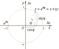
Trigonometric identities

Trigonometric functions are a way to link various lengths and angles in geometry. They are all based on observation of the so-called trigonometric circle:

One important aspect of the trigonometric functions is there inter-replationship. We are just going to list those but we are not going to demonstrate them. Let's consider this unit circle:

then:

$$ \begin{aligned} \sin \theta&= \frac{y}{h} \\\ \cos \theta&= \frac{x}{h} \\\ \tan \theta= \frac{\sin{\theta}}{\cos\theta}&=\frac{y}{x} \\\ \sin^2 \theta + \cos^2 \theta &= 1 \\\ \sin(\alpha + \beta)&=\sin \alpha \cos \beta + \cos \alpha \sin \beta \\\ \cos(\alpha + \beta)&=\cos \alpha \cos \beta - \sin \alpha \sin \beta \\\ \sin 2\theta &= 2\sin \theta \cos \theta \\\ \cos 2\theta &= \cos^2 \theta - \sin^2 \theta \end{aligned} $$

Some calculus

Notion of derivative

The base of calculus is derivation. Considering a continous function $f(x)$, the derivative of $f$ along its only variable $x$ is denoted:

$$ \frac{df}{dx}(x) $$

This represent the a function slope at $x$ of the function $f$. $dx$ represent a small nudge on the $x$ axis. The slope being effectively equal to:

$$ \frac{f(x+dx)-f(x)}{dx} $$

The smaller $dx$ is the better the approximation of the computation. Let's take $f(x)=x^2$. We know the slope at $0$ is $0$. Now let's use the formula above:

$$ \frac{df}{dx}(0)=\frac{f(x+0.001)-f(x)}{0.001}=0.00001/0.001=0.001 $$

So $0$ is not $0.001$ but it is close. And we can get arbitrarily closer as $dx$ becomes smaller:

$$ \frac{df}{dx}(0)=\frac{f(x+0.00001)-f(x)}{0.00001}=0.0000000001/0.001=0.00001 $$

As long as no computation is done, we can believe that dx is so small that it's value is negligible.

If we were to keep the formal definition, we would obtain the actual function which could be evaluated at every $x$:

$$ \begin{aligned} \frac{df}{dx}&=\frac{f(x+dx)-f(x)}{dx} \\\ &=\frac{(x+dx)^2-x^2}{dx} \\\ &=\frac{x^2+2xdx+dx^2-x^2}{dx} \\\ &=\frac{2xdx+dx^2}{dx} \\\ &=2x+\underbrace{dx}_{\text{very small so negligible}} \\\ &=2x \end{aligned} $$

Some basic derivative formula

As you can see we can find out the value of a derivative function by just applying the $f(x+dx) - f(x) / dx$ formula to any function really. The first thing we notive is that we can find a general rule for power of $x$:

$$ \frac{dx^n}{dx}=nx^{n-1} $$

So we can deduce what happens in the particular case $n=1$ or even $n=0$. The derivative of a constant is $0$. Indeed, a constant function as a flat slope.

What about $\sin$ and $\cos$? Well the demonstration are quite cumbersome so let's admit that:

$$ \begin{aligned} \frac{d}{dx}\cos x&=-\sin x \\\ \frac{d}{dx}\sin x&=cos x \end{aligned} $$

Meta-derivative

$$ \begin{array}{cc} \begin{aligned} (\alpha f+\beta g)^\prime&=\alpha f^\prime+\beta g^\prime && \text{(sum rule)} \\\ (f \cdot g)^\prime&= f^\prime g + fg^\prime && \text{(product rule)} \\\ (\frac{f}{g})^\prime&= \frac{f^\prime g - fg^\prime}{g^2} && \text{(quotien rule)} \\\ (f(g))^\prime&=f^\prime(g) \cdot f(g^\prime) && \text{(chain rule)} \\\ \end{aligned} \end{array} $$

Euler's number

Now what happens for function that looks like $a^x$ ? These functions are important because they appear a lot in real life applications. They basically represent physical phenomenon which state is propotional to the previous state as time is flowing.

As we get into the realm of time based function, let's call the function $a^t$. So let's try with $2^t$:

$$ \begin{aligned} f(t)&=2^t \\\ f^\prime (t)&=\frac{2^{t+dt}-2^t}{dt} \\\ &=\frac{2^t2^{dt}-2^t}{dt} \\\ &=2^t\frac{2^{dt} - 1}{dt} \end{aligned} $$

We end up with this $\frac{2^{dt} - 1}{dt}$ which seems hard to get rid of. Let's evaluate it with a small $dt=0.001$:

$$ \frac{2^{0.01} - 1}{0.01}=0.693387 $$

So:

$$ \frac{d2^t}{dt}\approx0.693387 \cdot 2^t $$

Let's try with $3^t$:

$$ \begin{aligned} \frac{d3^t}{dt}&=3^t\frac{3^{dt} - 1}{dt} \\\ &=3^t\frac{3^{0.001} - 1}{0.001} \\\ &\approx1.09922 \cdot 3^t \end{aligned} $$

So it seems function of the form $a^t$ have their derivative under the form of $ca^t$. But we can notice that when $a$ is between $2$ and $3$, the constant $c$ passes a very important step. It gets equal to $1$ at some point. Which is significant because it would mean that the derivative would be equal to the function. So let's assume a number $e\in ]2;3[$ for which $c=1$ so that:

$$ \frac{de^t}{dt}=e^t $$

This is the definition of euler's number. Whatever its value, which will calculate a little later, the important part is that it is equal to its own derivative. As a consequence:

$$ \frac{de^{ct}}{dt}=ce^ct \text{ (chain rule)} $$

Also, we can also find out a interesting property from the fact that the constant is one:

$$ \begin{aligned} \frac{e^{dt}-1}{dt}&=1 \\\ e^{dt}&=dt+1 \\\ e^0&=1 \end{aligned} $$

Because $dt$ can be made arbitrarily small.

Additionally, it worth noting the existence of another special function: $\ln$ which is defined by:

$$ a=e^{\ln(a)} $$

This is the definition of the natural logarithm. So $\ln(2)$ for example is $e^2$. Thanks to this function we are able to express any function of the form $a^t$ into the much more practical form $e^{\ln(a)t}$. So now we can quickly deduce how to calculate $\ln$ !

$$ \begin{aligned} \frac{d}{dt}2^t&=\frac{d}{dt}e^{\ln(2)t} \\\ 0.693387 \cdot 2^t &\approx \ln(2) e^{\ln(2)t} \\\ \ln(2) &\approx 0.693387 \end{aligned} $$

More generally:

$$ \ln(x)=\lim_{dt\to 0}\frac{x^{dt}-1}{dt} $$

Back to $e$. How do we compute its value? Not that this is any interesting per se, but at least it will be a good introduction to the taylor series.

Taylor series

Taylor series are a way to approximate a function with a polynomial at a particular point and with an abitrary precision. You will able to express any function, including $e^x$ by a polynomial of the form $P(x)=c_0+c_1x+c_2x^2+...c+nx^n+...$. In order to manage a finite term polynomial, let's note:

$$ P_n(x)=c_0+c_1x+c_2x^2+...c+nx^n $$

The higher the order, the more closly the polynomial will match the function but also the more costly it will be to actually do something useful about it.

How do we compute a taylor series? Let's take $\cos x$ at $x=0$ as an example. We want a polynomial whose value at 0 is $\cos(0)$. So it is fitting that $c_0=1$. The simplerst polynomial we can find then is $P_0(x)=1$. But this is true exactly at $0$. As soon as we start to look a little bit away from $0$ we can see the cosine is diverging from our simple function. So we can have a look a degree further and take the slope into account. We want the slope of our polynomial to be equal as the the slope of cosine at $0$, so:

$$ \begin{aligned} P_1^\prime (x) &= \frac{d}{dx}(\cos x)(0) \\\ c_1&=-sin(0) \\\ c_1 &= 0 \end{aligned} $$

So we still have $P_1(x)=1$. If we continue further for the second degree polynomial:

$$ \begin{aligned} P_2^{\prime\prime} (x) &= \frac{d^2}{dx}(\cos x)(0) \\\ \frac{d^2}{dx}(1+c_2x^2) &= -cos(0) \\\ 2c_2&=-1 \\\ c_2&=-\frac{1}{2} \end{aligned} $$

So $P_2(x)=1-\frac{1}{2}x^2$. $-sin(0)=0$ so $P_3(x)=P_2(x)$. One last round for $P_4$:

$$ \begin{aligned} P_4^{\prime\prime\prime\prime} (x) &= \frac{d^4}{dx}(\cos x)(0) \\\ \frac{d^4}{dx}(1+c_2x^2+c_4x^4) &= cos(0) \\\ 2\cdot 3 \cdot 4c_4&=1 \\\ c_4&=\frac{1}{4!} \end{aligned} $$

So finally $P_2(x)=1-\frac{1}{2}x^2+\frac{1}{4!}x^4$. Looking closely we can see a pattern here. In fact, we can define $P_n(x)$ as:

$$ cos(x)=\sum_{n=0}^{\infty}(-1)^n\frac{x^2n}{2n!} $$

Euler's number decomposition

What if we apply the same technique for Euler's number? Let's see:

$$ \frac{de^x}{dx}(0)=\frac{d^2e^x}{dx^2}(0)=...=\frac{d^ne^x}{dx^n}(0)=1 $$

So whatever $n$, $\frac{d^n}{dx}P(x)$ has to be equal to $1$.

$$ \begin{aligned} c_0 &= 1 \\\ c_1 &= 1 \\\ c_2 &= \frac{1}{2} \\\ c_2 &= \frac{1}{6} \\\ \vdots \\\ c_n &= \frac{1}{n!} \\\ \end{aligned} $$

So in the end, Taylor is telling us:

$$ e^x=1+x+\frac{1}{2}x^2+...+\frac{1}{n!}x^n+...=\sum_{0}^{\infty}\frac{x^n}{n!} $$

Complex numbers

Definition

A complex number is a number made out of two parts:

1. a real part, which belongs to $\mathbb{R}$ and
2. an imaginary part, which any $c\in\mathbb{R}$ multiplying the imaginary number $i$.

The imaginary number as the following property:

$$ i^2=-1 $$

Do not adjust your glasses. You read that well.

A typical complex number will be written:

$$ 2+5i $$

The set to which the complex numbers belong is denoted $\mathbb{C}$.

The way those numbers are represented usually is on the complex plane:

Addition works the same way on complex numbers, except that it operates on the real and imaginary part separatly:

$$ (3+5i)+(4-3i)=7+2i $$

Multiplication is distributed:

$$ \begin{aligned} (a+bi)\cdot(c+di)&=ac+abi+bci-bd \\\ &=(ac-bd)+(ab+bc)i \end{aligned} $$

Associated to a complex number $z$ is its conjugate, which is denoted $\bar{z}$:

$$ \begin{aligned} z&=3+5i \\\ \bar{z}&=3-5i \end{aligned} $$

The conjugate just revert the imaginary part. On the complex plane it means it is going to have the same "x coordinates" but will be symmetrix along the "x axis".

As a consequence, $z+\bar{z}$ is a real number. Indeed, the imaginary part is cancelled out. And $z\bar{z}$ is also a real number.

So what's the point of complex numbers? Well they can sometimes appear as root of some class of polynomials. For example:

$$ \begin{aligned} x^2+1&=0 \\\ x^2&=-1\\\ x=i &\text{ and } x=-i \end{aligned} $$

$x=-i$ because $(-i)^2=-1$ too.

Finally, what about $\frac{1}{z}$?

$$ \frac{1}{z}=\frac{\bar{z}}{\bar{z}{z}}=\frac{a-ib}{a^2+b^2} $$

Note that is $z$ is on the unit circle, then $a^2+b^2=1$ so effectively:

$$ \frac{1}{z}=\bar{z} $$

Which is to say that $\frac{1}{e^{i\theta}}=e^{-i\theta}$, but we knew that already.

Unit circle (again)

The way to represnt the complex plane usually involves the unit circle. Indeed there is a lot of affinity between the complex numbers and trigonometry:

The x axis is the real part and the y axis is the imaginary part. Very often, complex numbers are not allowed to wander off the unit circle and will be "normed" to fit on it. For example, instead of manipulating $1+i$, we will be dealing with $\frac{1}{\sqrt{2}}+\frac{1}{\sqrt{2}}i$, which will be on the same line but will lie on the unit circle.

You may have noticed that the multiplication of two complex numbers is quite ugly. Ending with all those multiplications. There is an another way to represent a complex number and it is under the form of polar coordinates. Under that form, a complex number is represented by its angle $\theta$ and its length $\rho$ (thank you trigonometry reminder):

$$ \begin{aligned} z=a+bi&=\rho\cos\theta+\rho i\sin\theta \\\ &=\rho(\cos\theta+i \sin\theta)\\\ \end{aligned} $$

Incidentally:

$$ \begin{aligned} a&=\rho\cos\theta \\\ b&=\rho\sin\theta \end{aligned} $$

So if we multyply two complex numbers:

$$ \begin{aligned} (a+bi)\cdot(c+di)&=\rho_1(\cos\theta_1+i \sin\theta_1)\cdot(\rho_2(\cos\theta_2+i \sin\theta_2) \\\ &=\rho_1\rho_2(\cos(\theta_1+\theta_2)+i \sin(\theta_1+\theta_2) \end{aligned} $$

In the middle there we did some magical trigonometry tricks. As you can see the number are added and the length multiply each other. So in a few words, "angles add, numbers multiply" when multiplying complex number.

What if we are on the unit circle now? Well all the $\rho$s are one. So multiplying is really rotating aroung the unit circle.

Eurler and complex, back to the title

So now we are ready to introduce $e$. Remember the taylor decomposition?

$$ \begin{aligned} e^{i\theta} &=1+i\theta+\frac{1}{2}(i\theta)^2+\frac{1}{6}(i\theta)^3+...+\frac{1}{n!}(i\theta) ^n+...\\\ &=1+i\theta-\frac{1}{2}\theta^2-\frac{1}{6}i\theta^3... \end{aligned} $$

Remember that $i^3=i^2i=-i$. Let's regroup the real part and the imaginary part:

$$ \begin{aligned} e^{i\theta} &=\underbrace{1-\frac{1}{2}\theta^2+\frac{1}{24}\theta^4}_{\text{taylor of}\cos \theta}+...+i(\underbrace{\theta-\frac{1}{6}\theta^3+...}_{_{\text{taylor of}\sin \theta}}) \end{aligned} $$

Crazy right? So we end up with:

$$ e^{i\theta}=\cos\theta+i\sin\theta $$

Which is the polar form of a complex number of norm $1$ (i.e. on the unit circle). Boom.

Note that we can represent all the complex numbers with this form, not only the complex numbers on the unit circle. We just need a multiplier:

$$ \rho e^{i\theta} $$

Thanks to the power rule, we now see clearly why numbers multiply and angles add:

$$ (\rho e^{i\theta})^r=\rho^n e^{in\theta} $$

This is where we introduce the root of 1. The one that solves $z^n=1$. Imagine the unit cicrle as a pie separated in $n$ equal sized parts. Each time a cut line crosses the unit circle we have a root for the equation. Let's $\omega_k$ be the nth root:

$$ \omega_k=e^{i\frac{2\pi}{k}} $$

Conclusion

So, what's $i^i$ ? Well

$$ \begin{aligned} i^i&=\underbrace{\cos \theta}_{\text{should be 0}} + (i\underbrace{\sin \theta}_{\text{should be 1}})^i \\\ &=\cos\frac{\pi}{2}+(i\sin\frac{\pi}{2})^i \\\ &=(e^{i\frac{\pi}{2}})^i \\\ &=e^{i^{2}\frac{\pi}{2}} \\\ i^i&=e^{-\frac{\pi}{2}} \end{aligned} $$

Cheers!