rayshade_maps_gg.R

#Rayshader reprex to try and put a flat raster map under a 
#set of 3d points
library(rayshader)
library(ggplot2)
library(dplyr)
library(maps)
library(ggmap)

data(world.cities)

japan <- world.cities %>% filter(country.etc == "Japan") %>%
  filter(pop > 1e6)
japan_map <- get_stamenmap(bbox = c(left = min(japan$long),
                           bottom = min(japan$lat),
                           right = max(japan$long)+3,
                           top = max(japan$lat)+3),
                           maptype = "watercolor",
                           zoom = 5)

#plot together
together_plot <- ggmap(japan_map) +
  geom_point(data = japan, 
             aes(x = long, y = lat, color = pop)) +
  scale_color_viridis_c(option = "C")

#Separate plots
map_plot <- ggmap(japan_map)

point_plot <- ggplot() +
  geom_point(data = japan, 
             aes(x = long, y = lat, color = pop)) +
  scale_color_viridis_c(option = "C")

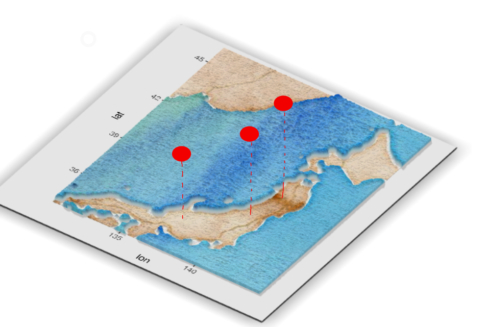
#together
plot_gg(together_plot,multicore=TRUE,
        width=4,
        height=4,
        scale=250,
        windowsize = c(1000,800))

render_camera(zoom = 0.5, theta = 130, phi = 35)
render_snapshot("together.png")

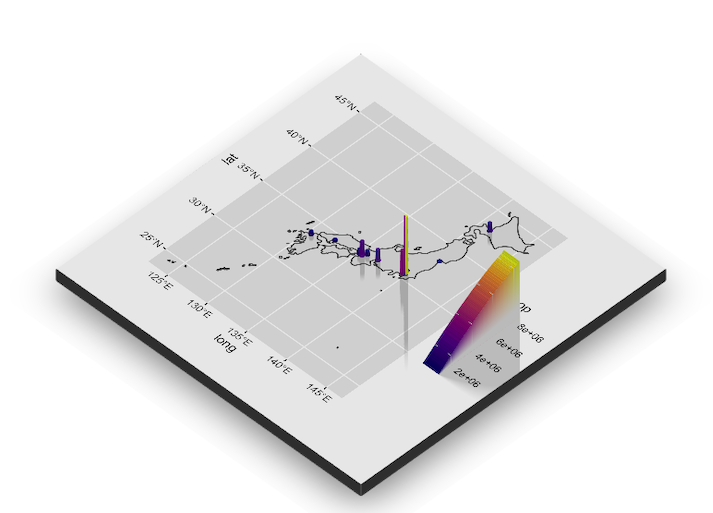
#Apart
plot_gg(list(map_plot, point_plot),multicore=TRUE,
        width=4,
        height=4,
        scale=250,
        windowsize = c(1000,800))

render_camera(zoom = 0.5, theta = 130, phi = 35)
render_snapshot("apart.png")

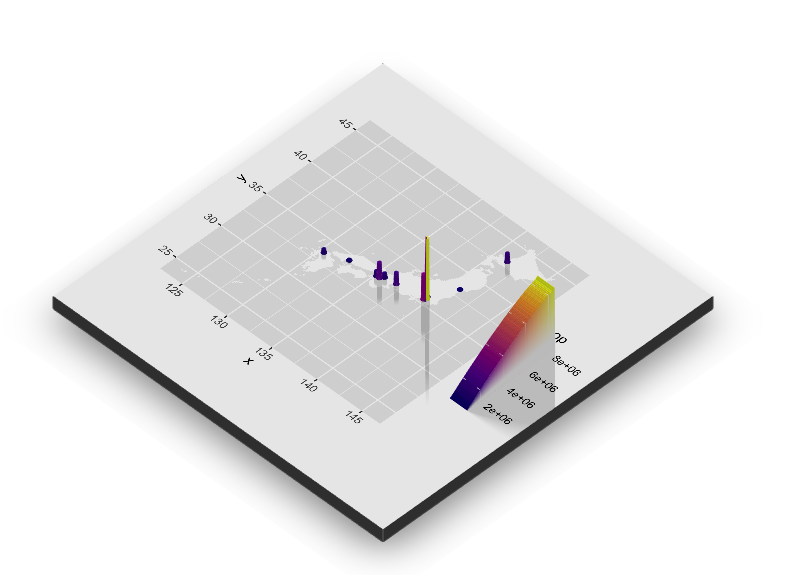
#apart2
plot_gg(list(point_plot, map_plot),multicore=TRUE,
        width=4,
        height=4,
        scale=250,
        windowsize = c(1000,800))

render_camera(zoom = 0.5, theta = 130, phi = 35)
render_snapshot("apart2.png")

  

OK, cool. So the basic point is to blank out the layer you want flat in one ggplot? Let's see if this holds in general for a polygon...

library(sf)

japan_poly <- sf::st_as_sf(map("world", plot = FALSE, fill = TRUE)) %>%
  filter(ID=="Japan")

#A plot we want to see
point_plot_poly <- ggplot() +
  geom_sf(data = japan_poly) +
  geom_point(data = japan, 
             aes(x = long, y = lat, color = pop)) +
  scale_color_viridis_c(option = "C")


#A plot with japan blanked out, but included
together_plot_poly <- ggplot() +
  geom_sf(data = japan_poly, alpha = 0, color = NA, fill = NA) +
  geom_point(data = japan, 
             aes(x = long, y = lat, color = pop)) +
  scale_color_viridis_c(option = "C")


#combine!
plot_gg(list(point_plot_poly,together_plot_poly),multicore=TRUE,
        width=4.5,
        height=4.5,
        scale=250,
        windowsize = c(1000,800))

YES!

Note, I initially tried this with just alpha = 0, but, didn't work - really needed to blank the whole thing.

Works for rasters, too!

Make a raster from the polygon

library(raster)
library(fasterize)
ref_rast <- raster(japan_poly, res = 0.1)
japan_rast <- fasterize(japan_poly, raster = ref_rast)

Use RStoolbox to plot the raster

library(RStoolbox)

#A plot we want to see
point_plot_rast <- ggR(japan_rast) +
  geom_point(data = japan, 
             aes(x = long, y = lat, color = pop)) +
  scale_color_viridis_c(option = "C")


#A plot with japan blanked out, but included
together_plot_rast <- ggR(japan_rast, alpha = 0) +
  geom_point(data = japan, 
             aes(x = long, y = lat, color = pop)) +
  scale_color_viridis_c(option = "C")



plot_gg(list(point_plot_rast,together_plot_rast),multicore=TRUE,
        width=4.5,
        height=4.5,
        scale=250,
        windowsize = c(1000,800))

Nice example @tylermorganwall .

I've been trying to plot a similar image with a slightly different approach: instead of showing geom_points() as "bars" in the 3d plot, I'm trying to use floating points. Do you have any thoughts on how I can do it?