You signed in with another tab or window. Reload to refresh your session.You signed out in another tab or window. Reload to refresh your session.You switched accounts on another tab or window. Reload to refresh your session.Dismiss alert
sequenceDiagram
participant User
participant Runner
participant SessionService
participant LlmAgent
participant LLM
participant MyTool
activate Runner
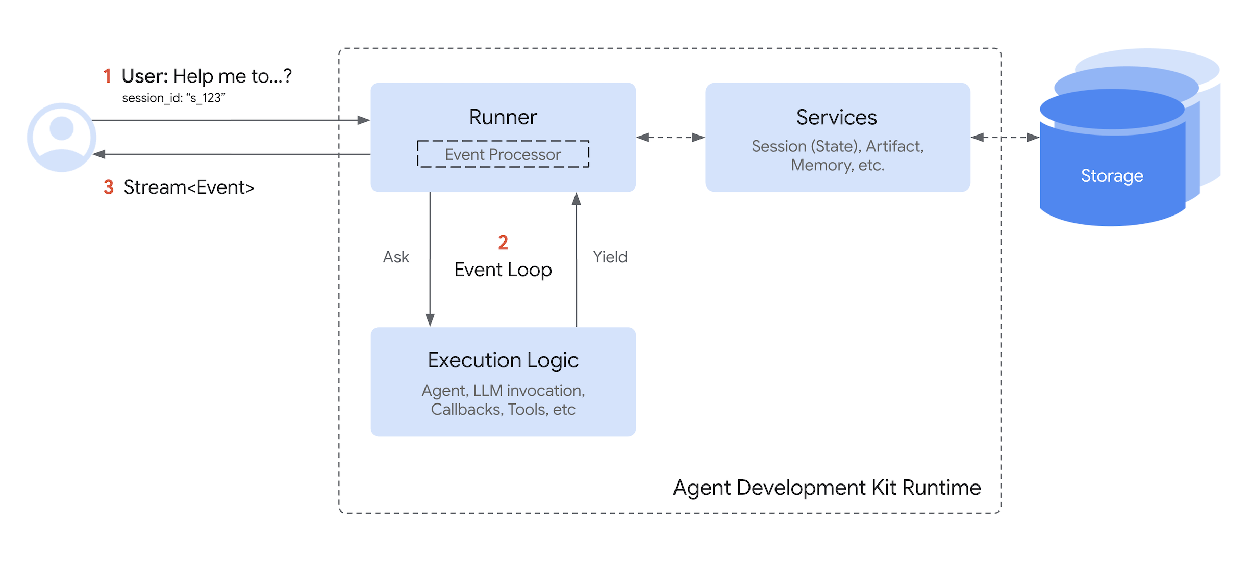
Note right of Runner: https://google.github.io/adk-docs/runtime/#runners-role-orchestrator
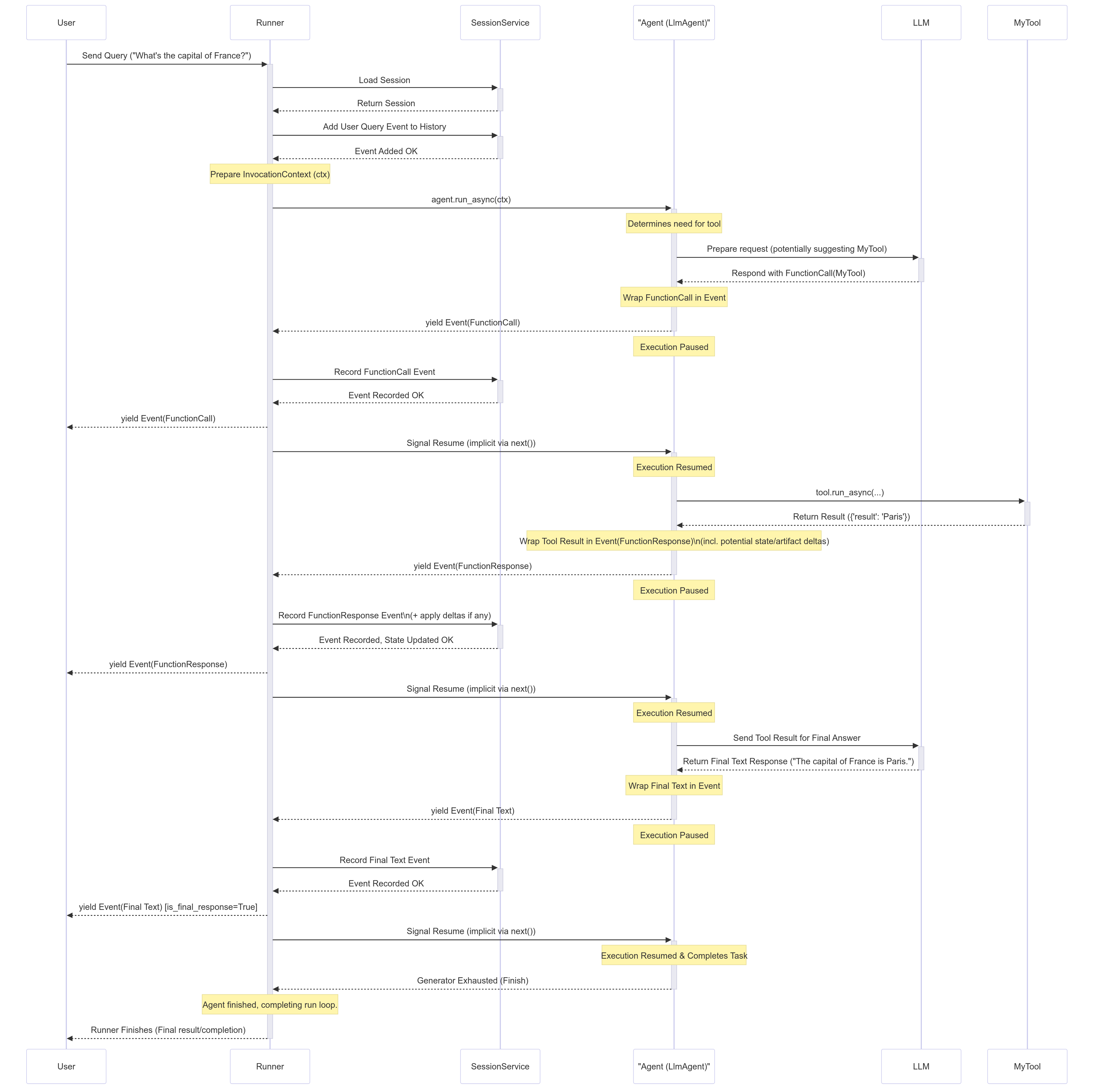
User->>Runner: send query ("what's the capital of France?")
activate SessionService
Runner->>SessionService: load Session
SessionService-->>Runner: return Session
deactivate SessionService
Note right of SessionService: https://google.github.io/adk-docs/sessions/session/
activate SessionService
Runner->>SessionService: Add user query Event to History
SessionService-->>Runner: Event added OK
deactivate SessionService
Note right of Runner: prepare InvocationContext(ctx)
activate LlmAgent
Runner->>LlmAgent: agent.run_async(ctx)
Note right of LlmAgent: determine need for tool
activate LLM
LlmAgent->>LLM: prepare request (potentially suggesting MyTool)
LLM-->>LlmAgent: respond with FunctionCall(MyTool)
deactivate LLM
Note right of LlmAgent: wrap FunctionCall in Event
LlmAgent-->>Runner: yield Event(FunctionCall)
deactivate LlmAgent
Note right of LlmAgent: execution paused
activate SessionService
Runner->> SessionService: record FunctionCall Event
SessionService-->>Runner: Event recorded OK
deactivate SessionService
Runner->>User: yield Event(FunctionCall)
activate LlmAgent
Runner->> LlmAgent: signal resume(implicit via next())
Note right of LlmAgent: execution resumed
activate MyTool
LlmAgent->>MyTool: tool.run_async()
MyTool-->>LlmAgent: return result({'result':'Paris'})
deactivate MyTool
Note right of LlmAgent: warp too result in Event(FunctionResponse incl. potential state/artifact deltas)
LlmAgent-->>Runner: yield Event(FunctionResponse)
deactivate LlmAgent
Note right of LlmAgent: execution paused
activate SessionService
Runner->>SessionService: record FunctionResponse Event plus apply deltas if any
SessionService-->>Runner: Event recorded, State updated OK
deactivate SessionService
Runner->>User: yield Event(FunctionResponse)
activate LlmAgent
Runner->>LlmAgent: signal resume (implicit via next())
Note right of LlmAgent: execution resumed
activate LLM
LlmAgent->>LLM: send tool result for final answer
LLM-->>LlmAgent: return final text response("The capital of France is Paris")
deactivate LLM
Note right of LlmAgent: warp final text in Event
LlmAgent--> Runner: yield Event(final text)
deactivate LlmAgent
Note right of LlmAgent: execution paused
activate SessionService
Runner->>SessionService: record final text Event
SessionService-->>Runner: Event recorded OK
deactivate SessionService
Runner->>User: yield Event(final text)[is_final_response=True]
activate LlmAgent
Runner->>LlmAgent: signal resume(implicit via next())
Note right of LlmAgent: execution resumed and completes task
LlmAgent-->Runner: generator exhausted(Finish)
Note right of Runner: Agent finished, completing run loop
deactivate LlmAgent
Runner-->User: Runner finishes (final result/conpletion)
deactivate Runner
Loading
Enriched
sequenceDiagram
    participant User
    participant main
    participant SessionService
    participant MemoryService
    participant Runner
    participant FunctionTool
    participant LlmAgent
    participant LLM
    participant MyTool

activate main

    main->>SessionService: instantiate with SessionService()

    main->>MemoryService: instantiate with MemoryService()

    activate Runner
        Note right of Runner: https://google.github.io/adk-docs/runtime/#runners-role-orchestrator

        main->>Runner: instantiate with Runner(..., session_service=session_service, memory_service=memory_service)

        User->>Runner: send query ("what's the capital of France?")
        Note right of Runner: ...

        activate SessionService

            Runner->>SessionService: load Session
            SessionService-->>Runner: return Session

        deactivate SessionService

        Note right of SessionService: https://google.github.io/adk-docs/sessions/session/

        activate SessionService

            Runner->>SessionService: Add user query Event to History
            SessionService-->>Runner: Event added OK

        deactivate SessionService

        Note right of Runner: prepare InvocationContext(ctx)

        activate FunctionTool

            Runner->>FunctionTool: instantiate with function name
            FunctionTool-->>Runner: object created

        deactivate FunctionTool

        activate LlmAgent

            Runner->>LlmAgent: instantiate with Agent(...,tools=[FunctionTool], output_key=$str)
            Runner->>LlmAgent: agent.run_async(ctx)
            Note right of LlmAgent: determine need for tool

                activate LLM

                    LlmAgent->>LLM: prepare request (potentially suggesting MyTool)
                    LLM-->>LlmAgent: respond with FunctionCall(MyTool)

                deactivate LLM

            Note right of LlmAgent: wrap FunctionCall in Event
            LlmAgent-->>Runner: yield Event(FunctionCall)

        deactivate LlmAgent

        Note right of LlmAgent: execution paused

        activate SessionService

            Runner->> SessionService: record FunctionCall Event
            SessionService-->>Runner: Event recorded OK

        deactivate SessionService

        Runner->>User: yield Event(FunctionCall)


        activate LlmAgent

            Runner->> LlmAgent: signal resume(implicit via next())
            Note right of LlmAgent: execution resumed

            activate MyTool

                LlmAgent->>MyTool: tool.run_async()
                MyTool->>SessionService: manage State via ToolContext.state.get($key) or ToolContext.state[$key]=$val
                MyTool-->>LlmAgent: return result({'result':'Paris'})

            deactivate MyTool

            Note right of LlmAgent: warp too result in Event(FunctionResponse incl. potential state/artifact deltas)
            LlmAgent-->>Runner: yield Event(FunctionResponse)

        deactivate LlmAgent

        Note right of LlmAgent: execution paused

        activate SessionService

            Runner->>SessionService: record FunctionResponse Event plus apply deltas if any
            SessionService-->>Runner: Event recorded, State updated OK

        deactivate SessionService

        Runner->>User: yield Event(FunctionResponse)

        activate LlmAgent

            Runner->>LlmAgent: signal resume (implicit via next())
            Note right of LlmAgent: execution resumed

            activate LLM

                LlmAgent->>LLM: send tool result for final answer
                LLM-->>LlmAgent: return final text response("The capital of France is Paris")

            deactivate LLM

            Note right of LlmAgent: warp final text in Event

            LlmAgent--> Runner: yield Event(final text)

        deactivate LlmAgent

        Note right of LlmAgent: execution paused

        activate SessionService

            Runner->>SessionService: record final text Event
            SessionService-->>Runner: Event recorded OK

        deactivate SessionService

        Runner->>User: yield Event(final text)[is_final_response=True]

        activate LlmAgent

            Runner->>LlmAgent: signal resume(implicit via next())
            Note right of LlmAgent: execution resumed and completes task
            LlmAgent-->Runner: generator exhausted(Finish)
            Note right of Runner: Agent finished, completing run loop

        deactivate LlmAgent

        Runner-->User: Runner finishes (final result/conpletion)

    deactivate Runner

deactivate main
At the validation stage, models with few or no hyperparameters are straightforward to validate and tune. Thus, a relatively small dataset should suffice.
In contrast, models with multiple hyperparameters require enough data to validate likely inputs. CV might be helpful in these cases, too. Generally, apportioning 80 percent of the records to train, 10 percent to validate, and 10 percent to test scenarios ought to be a reasonable initial split.
Variables of interest in an experiment (those that are measured or observed) are called response or dependent variables. Other variables in the experiment that affect the response and can be set or measured by the experimenter are called predictor, explanatory, or independent variables.
For example, you might want to determine the recommended baking time for a cake recipe or provide care instructions for a new hybrid plant.
Subject
Possible predictor variables
Possible response variables
Cake recipe
Baking time, oven temperature
Moisture of the cake, thickness of the cake
Plant growth
Amount of light, pH of the soil, frequency of watering
Size of the leaves, height of the plant
A continuous predictor variable is sometimes called a covariate and a categorical predictor variable is sometimes called a factor. In the cake experiment, a covariate could be various oven temperatures and a factor could be different ovens.
Usually, you create a plot of predictor variables on the x-axis and response variables on the y-axis.
Machine learning offers a fantastically powerful toolkit for building complex systems quickly. This paper argues that it is dangerous to think of these quick wins as coming for free. Using the framework of technical debt, we note that it is remarkably easy to incur massive ongoing maintenance costs at the system level when applying machine learning. The goal of this paper is highlight several machine learning specific risk factors and design patterns to be avoided or refactored where possible. These include boundary erosion, entanglement, hidden feedback loops, undeclared consumers, data dependencies, changes in the external world, and a variety of system-level anti-patterns.
├── LICENSE
├── Makefile           <- Makefile with commands like `make data` or `make train`
├── README.md          <- The top-level README for developers using this project.
├── data
│   ├── external       <- Data from third party sources.
│   ├── interim        <- Intermediate data that has been transformed.
│   ├── processed      <- The final, canonical data sets for modeling.
│   └── raw            <- The original, immutable data dump.
│
├── docs               <- A default Sphinx project; see sphinx-doc.org for details
│
├── models             <- Trained and serialized models, model predictions, or model summaries
│
├── notebooks          <- Jupyter notebooks. Naming convention is a number (for ordering),
│                         the creator's initials, and a short `-` delimited description, e.g.
│                         `1.0-jqp-initial-data-exploration`.
│
├── references         <- Data dictionaries, manuals, and all other explanatory materials.
│
├── reports            <- Generated analysis as HTML, PDF, LaTeX, etc.
│   └── figures        <- Generated graphics and figures to be used in reporting
│
├── requirements.txt   <- The requirements file for reproducing the analysis environment, e.g.
│                         generated with `pip freeze > requirements.txt`
│
├── setup.py           <- Make this project pip installable with `pip install -e`
├── src                <- Source code for use in this project.
│   ├── __init__.py    <- Makes src a Python module
│   │
│   ├── data           <- Scripts to download or generate data
│   │   └── make_dataset.py
│   │
│   ├── features       <- Scripts to turn raw data into features for modeling
│   │   └── build_features.py
│   │
│   ├── models         <- Scripts to train models and then use trained models to make
│   │   │                 predictions
│   │   ├── predict_model.py
│   │   └── train_model.py
│   │
│   └── visualization  <- Scripts to create exploratory and results oriented visualizations
│       └── visualize.py
│
└── tox.ini            <- tox file with settings for running tox; see tox.readthedocs.io
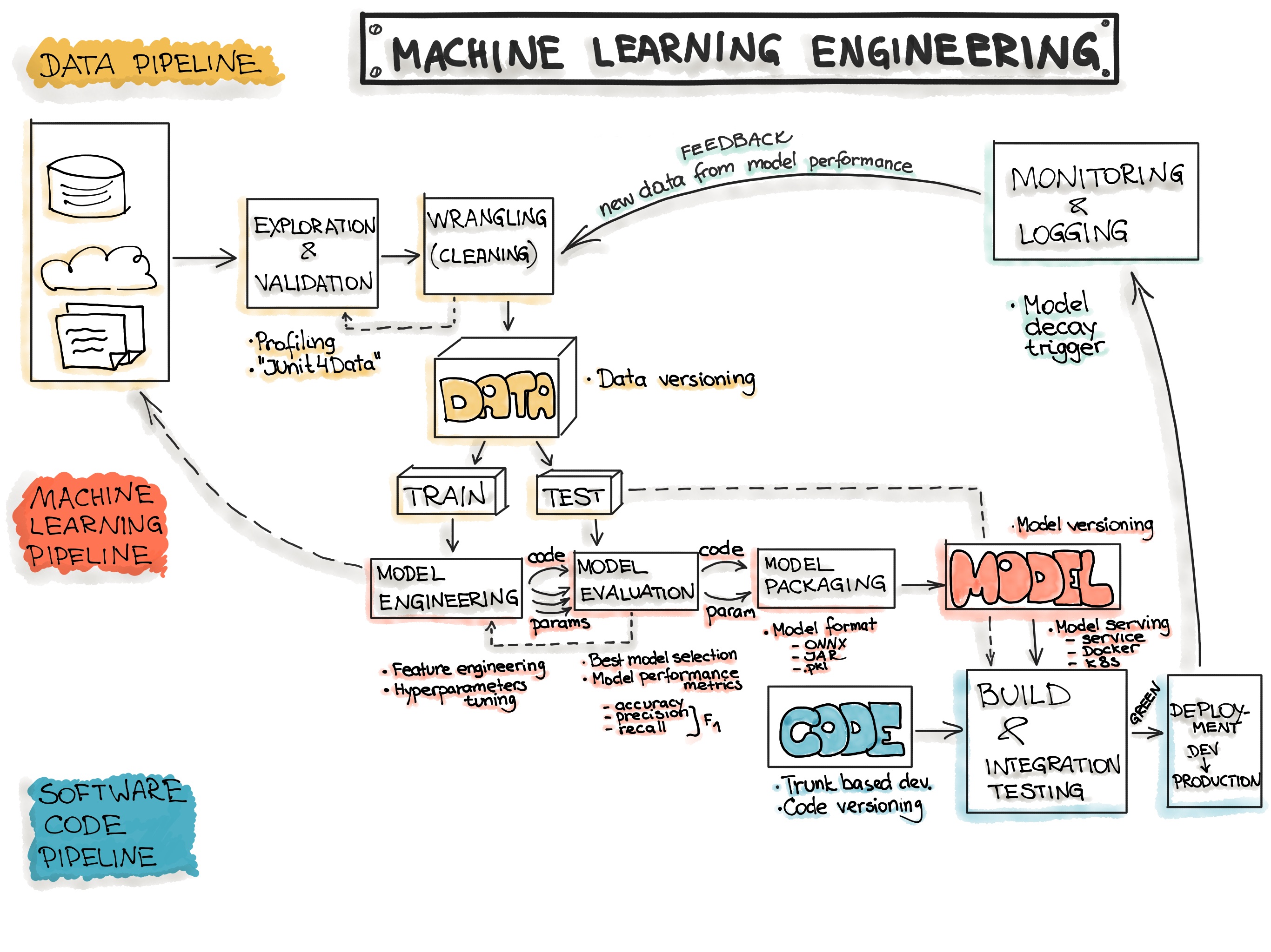
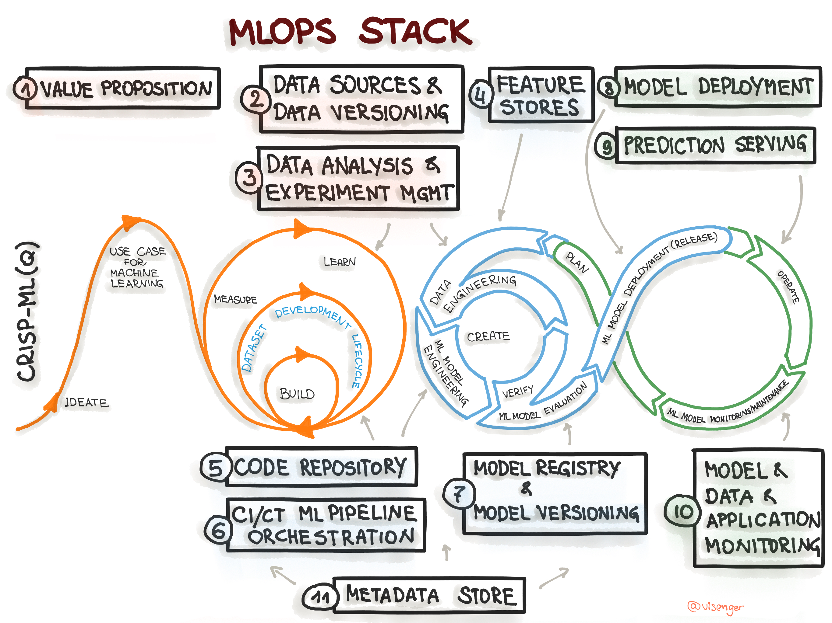
With Machine Learning Model Operationalization Management (MLOps), we want to provide an end-to-end machine learning development process to design, build and manage reproducible, testable, and evolvable ML-powered software.
Data Ingestion - Collecting data by using various frameworks and formats, such as Spark, HDFS, CSV, etc. This step might also include synthetic data generation or data enrichment.
Exploration and Validation - Includes data profiling to obtain information about the content and structure of the data. The output of this step is a set of metadata, such as max, min, avg of values. Data validation operations are user-defined error detection functions, which scan the dataset in order to spot some errors.
Data Wrangling (Cleaning) - The process of re-formatting particular attributes and correcting errors in data, such as missing values imputation.
Data Labeling - The operation of the Data Engineering pipeline, where each data point is assigned to a specific category.
Data Splitting - Splitting the data into training, validation, and test datasets to be used during the core machine learning stages to produce the ML model.
Model Engineering
Model Training - The process of applying the machine learning algorithm on training data to train an ML model. It also includes feature engineering and the hyperparameter tuning for the model training activity.
Model Evaluation - Validating the trained model to ensure it meets original codified objectives before serving the ML model in production to the end-user.
Model Testing - Performing the final “Model Acceptance Test” by using the hold backtest dataset.
Model Packaging - The process of exporting the final ML model into a specific format (e.g. PMML, PFA, or ONNX), which describes the model, in order to be consumed by the business application.
Model Deployment
Model Serving - The process of addressing the ML model artifact in a production environment.
Model Performance Monitoring - The process of observing the ML model performance based on live and previously unseen data, such as prediction or recommendation. In particular, we are interested in ML-specific signals, such as prediction deviation from previous model performance. These signals might be used as triggers for model re-training.
Model Performance Logging - Every inference request results in the log-record.
1) Data preparation pipelines 2) Features store 3) Datasets 4) Metadata
1) ML model training pipeline 2) ML model (object) 3) Hyperparameters 4) Experiment tracking
1) Application code 2) Configurations
Testing
1) Data Validation (error detection) 2) Feature creation unit testing
1) Model specification is unit tested 2) ML model training pipeline is integration tested 3) ML model is validated before being operationalized 4) ML model staleness test (in production) 5) Testing ML model relevance and correctness 6) Testing non-functional requirements (security, fairness, interpretability)
1) Unit testing 2) Integration testing for the end-to-end pipeline
Automation
1) Data transformation 2) Feature creation and manipulation 1) Data engineering pipeline 2) ML model training pipeline 3) Hyperparameter/Parameter selection
1) ML model deployment with CI/CD 2) Application build
Reproducibility
1) Backup data 2) Data versioning 3) Extract metadata 4) Versioning of feature engineering
1) Hyperparameter tuning is identical between dev and prod 2) The order of features is the same 3) Ensemble learning: the combination of ML models is same 4)The model pseudo-code is documented
1) Versions of all dependencies in dev and prod are identical 2) Same technical stack for dev and production environments 3) Reproducing results by providing container images or virtual machines
Deployment
1) Feature store is used in dev and prod environments
1) Containerization of the ML stack 2) REST API 3) On-premise, cloud, or edge
1) On-premise, cloud, or edge
Monitoring
1) Data distribution changes (training vs. serving data) 2) Training vs serving features
1) ML model decay 2) Numerical stability 3) Computational performance of the ML model
1) Predictive quality of the application on serving data
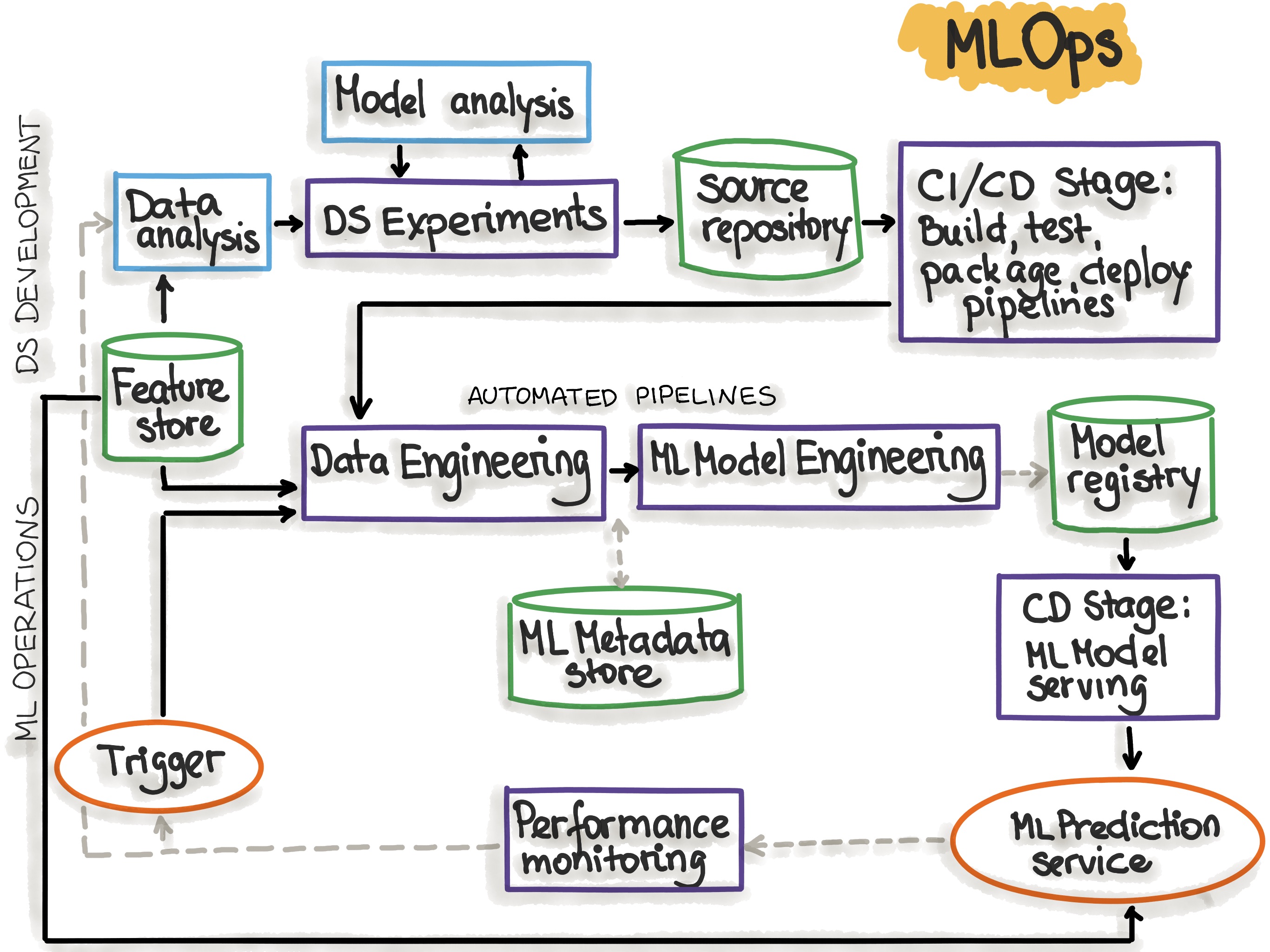
To specify an architecture and infrastructure stack for Machine Learning Operations, we suggest a general MLOps Stack Canvas framework designed to be application- and industry-neutral. We align to the CRISP-ML(Q) model and describe the eleven components of the MLOps stack and line them up along with the ML Lifecycle and the “AI Readiness” level to select the right amount of MLOps processes and technlogy components.
Figure 1. Mapping the CRISP-ML(Q) process model to the MLOps stack.
In the first course of Machine Learning Engineering for Production Specialization, you will identify the various components and design an ML production system end-to-end: project scoping, data needs, modeling strategies, and deployment constraints and requirements; and learn how to establish a model baseline, address concept drift, and prototype the process for developing, deploying, and continuously improving a productionized ML application.
Understanding machine learning and deep learning concepts is essential, but if you’re looking to build an effective AI career, you need production engineering capabilities as well. Machine learning engineering for production combines the foundational concepts of machine learning with the functional expertise of modern software development and engineering roles to help you develop production-ready skills.
Week 1: Overview of the ML Lifecycle and Deployment
Week 2: Selecting and Training a Model
Week 3: Data Definition and Baseline
Machine Learning Data Lifecycle in Production
In the second course of Machine Learning Engineering for Production Specialization, you will build data pipelines by gathering, cleaning, and validating datasets and assessing data quality; implement feature engineering, transformation, and selection with TensorFlow Extended and get the most predictive power out of your data; and establish the data lifecycle by leveraging data lineage and provenance metadata tools and follow data evolution with enterprise data schemas.
Understanding machine learning and deep learning concepts is essential, but if you’re looking to build an effective AI career, you need production engineering capabilities as well. Machine learning engineering for production combines the foundational concepts of machine learning with the functional expertise of modern software development and engineering roles to help you develop production-ready skills.
Week 1: Collecting, Labeling, and Validating data
Week 2: Feature Engineering, Transformation, and Selection
Week 3: Data Journey and Data Storage
Week 4: Advanced Data Labeling Methods, Data Augmentation, and Preprocessing Different Data Types
Machine Learning Modeling Pipelines in Production
In the third course of Machine Learning Engineering for Production Specialization, you will build models for different serving environments; implement tools and techniques to effectively manage your modeling resources and best serve offline and online inference requests; and use analytics tools and performance metrics to address model fairness, explainability issues, and mitigate bottlenecks.
Understanding machine learning and deep learning concepts is essential, but if you’re looking to build an effective AI career, you need production engineering capabilities as well. Machine learning engineering for production combines the foundational concepts of machine learning with the functional expertise of modern software development and engineering roles to help you develop production-ready skills.
In the fourth course of Machine Learning Engineering for Production Specialization, you will learn how to deploy ML models and make them available to end-users. You will build scalable and reliable hardware infrastructure to deliver inference requests both in real-time and batch depending on the use case. You will also implement workflow automation and progressive delivery that complies with current MLOps practices to keep your production system running. Additionally, you will continuously monitor your system to detect model decay, remediate performance drops, and avoid system failures so it can continuously operate at all times.
Understanding machine learning and deep learning concepts is essential, but if you’re looking to build an effective AI career, you need production engineering capabilities as well. Machine learning engineering for production combines the foundational concepts of machine learning with the functional expertise of modern software development and engineering roles to help you develop production-ready skills.
Week 1: Model Serving Introduction
Week 2: Model Serving Patterns and Infrastructures
Week 3: Model Management and Delivery
Week 4: Model Monitoring and Logging
The ‘Feature Store’ is an emerging concept in data architecture that is motivated by the challenge of taking ML applications into production. Technology companies like Uber and Gojek have published popular reference architectures and open source solutions, respectively, for ‘Feature Stores’ that address some of these challenges.
The concept of Feature Stores is nascent and we’re seeing a need for education and information regarding this topic. Most innovative products are now driven by machine learning. Features are at the core of what makes these machine learning systems effective. But still, many challenges exist in the feature engineering life-cycle. Developing features from big data is an engineering heavy task, with challenges in both the scaling of data processes and the serving of features in production systems.
Benefits of Feature Stores for ML
Track and share features between data scientists including a version-control repository
Process and curate feature values while preventing data leakage
Ensure parity between training and inference data systems
Serve features for ML-specific consumption profiles including model training, batch and real-time predictions
Accelerate ML innovation by reducing the data engineering process from months to days
Monitor data quality to rapidly identify data drift and pipeline errors
Empower legal and compliance teams to ensure compliant use of data
Bridging the gap between data scientists and data & ML engineers
Lower total cost of ownership through automation and simplification
Faster Time-To-Market for new model-driven products
Improved model accuracy: the availability of features will improve model performance
Improved data quality via data ->feature -> model lineage
The benchmarking was done on both an Nvidia DGX-1 and an IBM POWER Systems AC922 using a single GPU in each. The GPUs in the servers were both Nvidia V100 models, with the DGX-1 GPU having the model with 32GB of RAM and the AC922 having the 16GB model.
GDF Outperforms PDF
For time to load the input file, the GDF outperformed the PDF by an average of 8.3x faster (range 4.3x-9.5x). For the input file with 40 million records, the GDF was created and loaded in 5.87 seconds while the PDF took 56.03 seconds.
When sorting the data frame by values in one column, the GDF outperformed the PDF by an average of 15.5x faster (range 2.1x-23.4x). Due to the GPU in the AC922 only having 16GB of RAM, the 40 million row data frame was not able to be sorted so these number include the results of the sort on the DGX-1 for the 40 million row data frame.
When creating a new column that was populated with a calculated value, the GDF outperformed the PDF by an average of 4.8x faster (range 2.0x-7.1x).
The most remarkable performance difference was seen when dropping a single column. Amazingly, the GDP outperformed the PDF by an average of 3,979.5x faster (range 255.7x-9,736.9x). Performance scaled linearly as the size of the data frame became larger.
When concatenating the 631,726 row data frame onto another data frame, the GDF outperformed the PDF by an average of 10.4x faster (range 1.2x-29.0x). As with sorting, the 16GB GPU ran out of memory when trying to append the data frame onto the 40 million row data frame sorted so these number include the results of the sort on the DGX-1 for the 40 million row data frame.