Counting Crystals in Two Dimensions #research

research_two_dimensional_crystals.md

Table of Contents

1. 2D Materials from Programmable Matter
2. Using Symmetry to Count Configurations
   1. A Different Perspective on Symmetry
   2. Wyckoff Positions
   3. Suppressing the Combinatorial Explosion
   4. Sampling Crystal Structure Ensembles
3. Exploring Different Interactions
4. Optimizing the Exploration
5. Conclusions

tl;dr

This is an accompaniment to several manuscripts (text available upon request if you cannot access them):

1. "Using symmetry to elucidate the importance of stoichiometry in colloidal crystal assembly," N. A. Mahynski, E. Pretti, V. K. Shen, J. Mittal, Nature Commun. 10 2028 (2019). - Also see the ``Behind the paper'' post.
2. "Symmetry-based crystal structure enumeration in two dimensions," E. Pretti, V. K. Shen, J. Mittal, N. A. Mahynski, J. Phys. Chem. A 124, 3276–3285 (2020).
3. "Python Analysis of Colloidal Crystal Structures (PACCS)," E. Pretti, N. A. Mahynski, https://github.com/usnistgov/PACCS (2020).
4. "Grand canonical inverse design of multicomponent colloidal crystals," N. A. Mahynski, R. Mao, E. Pretti, V. K. Shen, J. Mittal, Soft Matter 16, 3187–3194 (2020).

In this series of papers we reconsidered the task of creating planar interfaces that require a unique surface pattern to be functional. In a system that self-assembles, such as an appropriate colloidal suspension, there are many possible configurations, but the one that we might hope to form spontaneously is the one with the lowest free energy. However, a ensemble of possibilities needs to be generated in order to screen them and establish which is the most thermodynamically stable one. To this end, we developed an algorithm, inspired by symmetry and the concept of orbifolds, that can enumerate point patterns as quickly as possible in two Euclidean dimensions. This enables the generation of different candidate patterns that are particularly relevant for atomic crystals made of atoms that are similar in size, or out of colloidal crystals made from similarly sized spherical constituents. This method enumerates structures according to rules of symmetry; compared to random searching, this enables the enumeration of "important" candidate structures is trillions of times faster, reducing a calculation that would otherwise take the age of the universe to complete (13.8e9 years) to a mere 15 minutes. This code is available in Ref. 3 above, and is further described in Ref. 2.

Many of the graphics below have been presented at scientific conferences including:

• "Symmetry-based discovery of multicomponent, two-dimensional colloidal crystals," N. A. Mahynski, E. Pretti, V. K. Shen, J. Mittal, American Physical Society March Meeting, Denver, CO USA (03/2021).
• "Symmetry-based discovery of multicomponent, two-dimensional colloidal crystals," N. A. Mahynski, E. Pretti, V. K. Shen, J. Mittal, GRC: Colloidal, Macromolecular & Polyelectrolyte Solutions, Ventura, CA USA (02/2020).
• "Grand canonical inverse design of multicomponent colloidal assemblies," N. A. Mahynski, E. Pretti, V. K. Shen, J. Mittal, American Institute of Chemical Engineers Annual Meeting, Orlando, FL USA (11/2019).
• "Symmetry-based discovery of multicomponent, two-dimensional colloidal crystals," N. A. Mahynski, E. Pretti, V. K. Shen, J. Mittal, American Institute of Chemical Engineers Annual Meeting, Pittsburgh, PA USA (11/2018).
• "Symmetry-based discovery of multicomponent, two-dimensional colloidal crystals," N. A. Mahynski, E. Pretti, V. K. Shen, J. Mittal, Foundations of Molecular Modeling and Simulation, Delavan, WI USA (07/2018).

Please cite appropriately if you find this material to be helpful.

2D Materials from Programmable Matter

Two dimensional materials play an important role in a number of scientific fields and engineering applications. For example, in creating responsive surface coatings, membranes with controllable porosity, or placing ligands to act as selective receptors for chemical separation or sensing tasks. In general, these surfaces are built from molecular, or macromolecular, units and so must be programmed to self-assemble rather than rely on an external agent or force to organize them if these materials are to be produced in large quantities. This chemical programming can potentially be achieved in a number of ways. If the constituents are colloidal (nano)particles, they may be functionalized with various ligands in isotropic or anisotropic ways, their shape may be tuned (e.g., spherical or non-spherical), or external directing agents such as additives or fields (e.g., electrical or flow/shear) may be applied. In the image below, the $\lambda$ values represent differently programmed interactions between the different pairs of colored spheres (blue-blue, blue-green, green-green), which spontaneously self-assemble into different structures based on (1) these values and (2) the ratio of the number of green to blue particles.

DNA has proven to be a powerful ligand whose specific, progammable interactions based on sequence can be leveraged to create exquisite nanoscale devices and structures, sometimes collectively referred to as "DNA nanotechnology." While DNA is not required, widespread interest has driven a great deal of research into it. A typical design approach is to take a spherical nanoparticle and graft a certain type (sequence) of single-stranded DNA, sometimes with an initial double stranded region for stability, to its surface. The number of different sequences and their arrangement on the surface (how the surface is "functionalized") control how the nanoparticle interacts with other nanoparticles, which may (or may not) be grafted with complementary strands that interact favorably creating an attraction between the two. It is also possible to simply use the strands directly to create "origami" structures or other frameworks via these specific interactions, as illustrated in the figure below from this paper by Chandrasekaran and Levchenko.

While it is sometimes intuitive to understand how to functionalize a nanoparticle to obtain a desired structure via self-assembly, often it is very difficult to do so. The tactic of "inverse design" is where one starts from a desired structure, such as one in the first image above, and works backwards to derive the interactions or funcationality that give this result (i.e., the $\lambda$ values). The more conventional "forward design" is the Edisonian "trial and error" methodology in which interactions are tested and tweaked to seek out the desired result in a generally iterative fashion. The latter is often how experiments proceed, however, via the application of theory and simulations one can proceed with the former. Inverse design methods have proven incredibly useful and been used to reverse engineer many structures. Generally this involves performing some sort of molecular simulation, such as molecular dynamics or Monte Carlo, measuring properties of the system to establish (1) the properties of the current configuration and (2) how we expect they will change in response to modifications to, e.g., functionality. The details vary, but step (2) informs you how to update your current state to get closer to your goal; this is iterated until a result that is sufficiently close is achieved.

A couple of issues tend to arise, in practice, when performing inverse design. First, is insufficient sampling. This may mean different things within the context of the specific approach being used, but generally the issue is that you have not explored enough candidate parameter space to choose the best point from. This can result from simulations not being run long enough, databases being too sparse, or a poor choice of a basis set of candidates. Even then, inverse design can often produce physically unrealizable results. For example, a shape of nanoparticle that we cannot synthesize or perhaps a pair interaction potential that we do not understand how to create via known chemistry. It is possible to reduce the search space to physically realizable realms, which is one way to help remedy this problem; unfortunately, this may mean that the space you confine yourself to does not contain a solution to creating the structure you want.

Another solution is to try to use many "simple" components instead of a single "complex" one; if we have designed a system to assemble into a strange configuration using only one building block, it is often the case that the interaction between those blocks that causes this will be equally "strange". For example, perhaps the potential contains unusual oscillations or has discontinuities, unlike a more "conventional" Lennard-Jones potential which is considered more tractable. Instead, we could try to achieve this complexity through diversity by using multiple simpler "lego"-like building blocks that have interactions more akin to Lennard-Jones. The issue that arises in that approach originates with Gibbs Phase Rule. The number of thermodynamically permissible phases grows linearly with the number of components. In practice, we want to engineer the functionality of the nanoparticle such that at the conditions of interest, e.g., room temperature and atmospheric pressure, the only stable phase is the one we are targeting. In principle, it is possible to have more than one which are stable and will coexist, which is usually not a desirable scenario. As the number of components, so too does the number of allowable phases increasing the chance that we will struggle to engineer the system to exist in only one of them. As an aside, phase separation is also a problem in molecular simulations since there are issues with nucleation due to the finite size and length of simulations making it hard to know if the system would phase separate if run for longer or in a larger simulation box; both of which are generally kept as small as possible to make the iterations of inverse design as quick as possible.

Using Symmetry to Count Configurations

A Different Perspective on Symmetry

Forward design also suffers from the problem of sparsity. Even if we look up 1 million different structures, evaluate their free energy using the chosen functionality, and predict the one with the lowest as our expectation of what will assemble, we cannot guarantee that those candidates contained the correct answer to begin with. This is the first challenge that must be addressed. Many current approaches follow along these lines by doing simulations to generate a set of plausible candidates, looking up structures in known databases, or doing some sort of other machine learning/data-driven approach to generate this list. In the end, none of these approaches are very systematic and could be biased by data availability (e.g., perhaps all structures in a database only have a certain set of symmetries) or by the method (simulation) itself.

It is possible to enumerate structures more systematically, however, this is almost never done in practice due to the "combinatorial explosion" of possibilities. If you discretize an area into $N^2$ pixels (or voxels in 3D) and try to fill half of them ($m=N^2/2$, i.e., a 1:1 ratio of 2 components), as shown on the right, the number of possible arrangements exceeds Avogadro's number (6.022e23) by the time the lattice is $8 \times 8$. If you counted these structures at 1 millions configurations per second that would take 6.022e17 seconds, or roughly the age of the universe (13.8e9 years = 4.35e17 seconds).

This number of seconds is also roughly equal to the number of arrangements of a $3\times3\times3$ Rubik's cube (4.3e19), so the task is within a few orders of magnitude of trying to count all of those configurations! However, clearly Rubik's cubes can be solved much more quickly if you know the right pattern and rules to achieve your target arrangement. So can we also be clever about how we count or arrange particles on our 2D lattice to achieve a similar speed up?

The answer is: yes. If we restrict ourselves to consider periodic crystals, then we are essentially looking for all ways to organize particles in all possible symmetries. In two Euclidean dimensions there are 4 isometries of the plane: translation, rotation, reflection, and glide reflection (reflection about a line, followed by translation along it). All unique combinations of these isometries represent symmetry groups, sometimes called "wallpaper groups" in 2D. There are only 17 wallpaper groups in 2D, which makes considering each of them individually tractable. While there are many ways to represent wallpaper groups and crystallographic symmetry, the conventional approach is to look at the fundamental domain (FD) or asymmetric unit of the crystal and use matrix operations to describe how symmetry makes copies of it. The FD is the smallest, generally simply connected, region of space that encloses no symmetry elements; you can view it as the smallest piece of the puzzle that the crystal is going to be formed by tesselation.

This focus on how operations move the "interior" of the FD around stands in contrast to the topological description of symmetry which instead focuses on the boundary. By "interior" I mean that the mathematical description uses matrices ("generators") like those found on the Bilbao crystallographic server to operate on the FD. However, when these symmetry operations occur, each FD touches copies of itself. These matches indicate symmetrically equivalent points. One consequence of this is that the boundaries of the FD are not all independent; in other words, if you view the space like a domain of numbers, e.g., [A, B), where we indicate the inclusivity of a bound by the chosen bracket symbol ("[" vs. ")") then there should be some equivalent to indicate the bounds of the FD. For example, if you repeat the p1 boundary conditions often used in molecular simulation (translate a rectangle up/down and left/right to repeat) then we should formally only include either the top or bottom in our FD, but not both. Explictly, the domain is $\mathcal{D} = \left[ x \in [0, L_x), y \in [0, L_y) \right]$. However, explicit consideration of this has not appeared until recently in computational packages used for crystallography despite this well-known shortcoming.

In contrast to generators (more "barycentric" in philosophy), if one focuses only on those equivalent boundaries, one arrives at an equivalent description of symmetry but which is "boundary-centric"; if you fold the FD to match all equivalent points you obtain a surface called a crystallographic orbifold. More information on the history and a more formal description of orbifolds can be found here. For example, in the figure above 3 different wallpaper groups are represented. p1 results by copying the rectangle left and right, and up and down; this means the top and bottom edge are equivalent, as are the left and right. Thus, we fold the rectangle to match them, which results in a torus. The cm group requires that we take the right edge and "flip" it to match the left, producing a Moebius band. A hybrid of the two results in pg, whose orbifold is a Klein bottle which results from "gluing" two Moebius bands together. Essentially, this means that boundary condition is related to symmetry. In some sense, this is analogous to the popular video game puzzle series "Portal" which is often cited as "one of the greatest video games ever made".

John H. Conway and William Thurston have shown that there is a unique orbifold for each wallpaper group, and Olaf Delgado-Friedrichs and Daniel Huson later showed that all possible FDs for a group can be derived by "cutting" the group's orbifold open so that it "falls flat" on the plane it represents. As this suggests, there are more than one possible FD for each group, sometimes instead called isohedral tiles. If we choose our FDs carefully, we can come up with a simple way to generate crystal patterns in an "even-handed" way. This is the essence of the algorithm we devised in Refs. 1-3 above. As shown in the figure at the left, we elect to create FDs by imagining them as rectangles, described by $L_1, L_2,$ and the angle $\alpha$. Different groups will have different restrictions on the ratio of the two edges and the value of $\alpha$, but when created as described in Refs. [1-2] all of the nodes created by crossing lines on the boundaries will map exactly to other ones. This means we can easily create a lattice consistent with the group's symmetry. Different groups have a different number of FDs per primitive cell, but if we bound the number of nodes, we can create lattices for each group that have similar node densities. This allows us to compare different lattices "fairly".

The general primitive cell in 2D is a parallelogram, but it is not obvious (at least to the author) that the FD should also follow the same prescription, especially given that the International Tables for Crystallography use very different shapes to describe the wallpaper groups. Upon rearrangement, however, they can be shown to be identical to those used in Refs. [1-2].

So what does this have to do with the "rules" used to solve a Rubik's cube and how can it help with the combinatorial explosion problem?

Wyckoff Positions

By virtue of the fact that the FD is bounded, and therefore does not wholly include points on its edges, and that symmetry implies some points are redundant, different positions along the boundary do not all "count" the same. All points in the interior of a FD belong to what is known as the "general Wyckoff position"; that is, we may assign those points a stoichiometric factor of "1" since they are entirely encompassed by the domain, whereas those on the edges may have values less than 1. Those positions on the edges which have values less than 1 are known as "special Wyckoff positions" - note that not all boundary points are "special", but all special positions are on the edge. In fact, an orbifold is essentially just a topological space with an embedded set that represents the Wyckoff sites; again, these are equivalent descriptions, but from different perspectives. The so-called "orbifolding" process simply bends and folds the FD at the these positions. Note that only rotations (cone points) and reflections (boundaries, including intersecting ones) encode special positions; p1 (o) and pg (xx) have only translations or glides and have only general positions and form platycosms in 2D! Check for yourself.

Consider the example below. In it, we consider a FD for the p6 (632 in orbifold notation) group where our domain is a triangle, as shown. The triangle is discretized into lattice points indicated by the light gray lines. Points on the edges are colored; those which are lighter (right half) are symmetrically equivalent to those on the left which are colored darker. You can see how this results from the primitive cell shown with the 6 FDs that compose it. In this case, only 10 independent nodes exist. Nodes such as the yellow, orange, and green ones would seem to only have "half" of themselves inside the domain; however, they get another "half" from their symmetrically equivalent position for a total factor of 1. The clear points in the middle also have a factor of 1. The red and purple sites have factors of 1/3 and 1/2, respectively, since this is the fraction they "sweep out" and "map" to themselves; that is, there are no other points to consider. Finally, the magenta point sweeps out and angle of $(2\pi)/12$ on the FD, but since there are 2 sites it has a net factor of 1/6. Note that in this case we have 3 special Wyckoff positions with factors of 1/6, 1/3, and 1/2 which correspond to its orbifold designation of "632". Generally, these factors are referred to as "site multiplicities" and are normalized by the smallest number so that the point with the lowest multiplicity (magenta) has a multiplicity of 1, while the largest (general positions) have a multiplicity of 6. More information can be found in Ref. [2].

We are the faced with the question: "how many ways can I place particles on this grid with a certain stoichiometric ratio?" In fact, this is essentially just a constraint satisfaction problem; this general class of problems describes many puzzles such as crosswords, sudoku, and even Rubik's cubes as shown in 2011 here. Note that this "CSP" should not be confused with the "crystal structure prediction" problem which has the same acronym and, in fact, is also what we are solving here!

Also, note that Rubik's cubes were originally called "magic cubes". Any relation to Conway's "Magic Theorem" surrounding orbifolds?!

By using modern computational CSP algorithms we can solve all possible ways to place particles on symmetrically distinct positions so that they result in a crystal with a given stoichiometric ratio. For example, to achieve a 1:2 ratio of blue to green particles we could place 1 green on a clear node in the middle and 1 blue on the purple node (1/2:1 = 1:2); we could also place 1 green and 2 blue particles on different clear nodes. In the first example, there are three ways to realize this because there are three different clear nodes to place the green particle. Similarly, the second example has $_3C_1 = 3!/(1!2!) = 3$ solutions depending on which site is chosen to host the lone blue particle. Obviously, this "puzzle" is underspecified, unlike the sudoku puzzles you will find newspapers or other airplane-based literature. The "solution index" in the histogram above essentially refers to which puzzle is being solved and the vertical axis to the number of possible solutions. The different ways of labeling the points based on their physical location (edges vs. corners vs. face scheme; orange histogram) or their net stoichiometric factor (Wyckoff multiplicity; blue histogram) is what defines "which puzzle" we are solving. Ultimately, it does not matter as the total number of solutions is identical (sum of the histograms). Each entry corresponds to a different solution and (usually) a different structure!

Importantly, note how stoichiometry is intrinsically linked to specific positions in the crystal. In the fluid phase of matter stoichometry is also more "fluid" in that it can change more continuously simply because we can add 1 more "blue" particle to a sea of "green" ones and it will simply diffuse about, not being fixed to one specific location. In crystals, while we can do something similar by adding particles to the general Wyckoff position, the special position is a unique concept specific to crystalline phases of matter. As a result, stoichiometry and symmetry are directly linked.

Suppressing the Combinatorial Explosion

Let's review the procedure to sample different possible crystal structure candidates (see Ref. [2] for more details), which can be viewed as traversing levels of a tree:

• [gray] Select an upper bound on the size of the primitive cell so we can "fairly" compare different groups,
• [orange] Choose a wallpaper group,
• Construct the FD grid based on the first 2 choices,
• [blue] Choose a stoichiometry (for any number of components, there is no upper bound),
• [green] Enumerate solutions to the CSP,
• Sample from these solutions.

The last step of "sampling" we will discuss a more later on. For now, let's reconsider the number of possible solutions to each CSP. In general, we do not consider p1 to be part of an interesting ensemble of structures. Because of its toroidal boundary conditions, we have no special Wyckoff positions in p1. This is the group with the "lowest" symmetry and it is used conventionally to simulate fluid phases of matter with molecular dynamics or Monte Carlo methods; note that this is usually acceptable since the unit or primitive cell of any crystal has p1 symmetry, so we can handle crystals by simply simulating a larger piece of it. In p1 the FD is equal to the primitive cell, whereas in all other groups the FD is between 1/2 - 1/12 of this size. For a $N \times N$ grid with p1 symmetry, we just have $(N-1) \times (N-1)$ independent sites with factors of 1 - the number of possibilities explode combinatorial just as before. This explosion happens for all groups; however, comparing unit cells of the same size, we have 1/2 or less the degrees of freedom (the FD) relative to p1. This means the number of possibilities is determined by choosing from less that $(N^2/2)$ not $N^2$, which dramatically "delays" the explosion until the cell would be much bigger.

Consider that if we wanted to enumerate all possible configuration of particles on a lattice. We might begin by writing a loop to place a blue particle in the first position, then have a second loop to place a green one in all the others one at a time. We could repeat for 2 or more green particles, and for multiple blue particles placed in different locations. Essentially, this is a giant "for" loop that would create many, many configurations. However, only a few would have "high" symmetry if we fortuitious placed everythiing "just so". Consider the p6 example at the left; if the particle highlighted in yellow was placed anywhere else, say the location indicated by magenta, the symmetry of the crystal would be destroyed. We essentially "downgrade" from p6 to p1. Our algorithm is able to directly propose the high symmetry structures, without having to loop over all possibilities then go back and determine which ones have a certain symmetry or not, allowing us to skip the defective one.

In principle, since these high symmetry crystals are found "by luck" in the loop described above, the "gap" between the dashed curve (enumerated by the PACCS code) and the solid line (combinatorial explosion of the equivalent p1 grid) contains all the "low" or "near" symmetry candidates; structures that are characterized by image above where we misplaced a single particle. Prof. David Wale's "high symmetry hypothesis" suggests that structures with high symmetry tend to have either very low or very high energies due to structural correlations. An approximate explanation is that symmetry repeats patterns; if we have a favorable local arrangement of particles (low energy) this is repeated and drives the energy; conversely, if we have a "bad" local arrangement the energy is driven upward because this is continuous repeated throughout the crystal. Structures with less symmetry repeat things less often (or not at all in p1) so you can some local arrangements that are "good" and some that are not, averaging out somewhere in the middle.

Thus, if we focus on high symmetry candidates only, we can get an ensemble of structures that contain either very good or very bad guesses as to what configuration represents the ground state (most stable state at low temperatures). This is an ansatz, but since this reduces the number of structures we need to consider from somthing like Avogadro's number (order of 1e23) for a unit cell of $N_g^2 = 8 \times 8$ (think crystals with roughly 64 atoms or colloids per unit cell) to roughly 1e9, the improvement is staggering. As previously stated, counting the former at 1e6 structures/sec would take longer than the age of the universe, whereas the latter would take only 15 minutes at the same rate! Telling which ones are "good" and which are "bad" is a simple matter of evaluating the energy, or relevant free energy.

Importantly, it is still not very reasonable to have a code that simply "dumps" out 1e9 structure to disk as even modern hard drives can be ovewhelmed by this operation. The code in Ref. 3 instead uses python generators which have essentially "memorized" the tree shown earlier for the problem at hand. In truth, because each next step in the tree is deterministic based on the symmetry (or symmetries) and stoichiometry chosen, and the sampling parameter (random number generator state) of the tree the code simply returns the next structure "in line" each time the generator is queried because it knows how to get to next leaf in the sequence. This makes the code deployable essentially regardless of the scale of the problem (upper bound on the size of the unit cell). Algorithmically, we can view the PACCS code in Ref. 2 as a black box which maps integers up to $N$ (when there are $N$ CSP solutions) to crystal structures. Sampling integers in a different order equates to a different structure ensemble if you sample from less than $N$ structures (complete enumeration).

The reason the combinatorial explosion is suppressed is ultimately three-fold:

• We are working with the fundamental domain (1/2 - 1/12 the size of the primitive cell) instead of the primitive cell.
• We have removed the degrees of freedom from redundant (symmetrically equivalent) boundaries.
• We have exploited the Wyckoff multiplicity explicitly to enumerate structures with targeted stoichiometries.

Sampling Crystal Structure Ensembles

Our algorithm allows us to directly and quickly generate crystalline candidates from whatever set of wallpaper groups and stoichiometries we may choose. However, it may not always be desirable to explicitly count all possible structures (e.g., if $N_g$ is large this does become intractable). Moreover, the generation routine up to this point still produces points on lattices, not in continuum space. It is generally preferrable to relax the latter in continuum using the chosen set of interactions between colloids or nanoparticles. This can be done with simple minimization, as well as other methods I will discuss next. Regardless, because we are generally going to relax these initial candidates later on, we can tolerate an incomplete lattice enumeration as long as the ensemble is reasonable.

Our algorithm enables us to sample the tree in a stochastic fashion if less than complete enumeration is desired. Following the analogy made earlier that the code essentially maps integers to strutures, we can simple choose integers in a different ways and generate different ensembles. But should this be done randomly, or can we be somewhat intelligent about it? Again, the answer is: yes. Consider the 7th figure above (the one with the Sudoku puzzle on it); on the lower half, structures from the left side of the histogram of CSP solutions seem to (my eye) be a bit less "complicated" than those on the right. The concept of a "complex" crystal vs. a "simple" one is a bit subjective, but we offered the following simplistic viewpoint in Ref. 2. If we considered a snapshot of an ideal gas configuration of particles (effectively randomly placed), there are essentially an infinite number of valid pairwise distances between different particles; this is true only if we look at a large snapshot, i.e., a very large "unit cell". Conversely, in a crystal there are many that are disallowed because particles are fixed at specific points in the crystal. We consider a crystal with a very "simple" structure to be one which has less of these different distances. Consequently, we could view the large snapshot of an ideal gas to be an infinitely "complex" crystal; this is consistent with other definitions of complexity which typically scale with the size of the primitive cell (larger cell means more complicated). Recall the ergodic hypothesis states a large spatial average is equivalent to a long term temporal average so for us to have a reasonably compete observation of "many" interparticle distances (which could be observed in a small simulation cell averaged over a long time), we can also look at a single snapshot of very large cell. This very large equates with complexity. Intuitively, it is clear that if you considered the ideal gas snapshot to be a crystal, you have many particles all held together in seemingly random positions - in order to achieve that the interparticle potential is likely to be very complicated, indeed.

We can then quantify this complexity by taking the (Kullback-Liebler) divergence, $D_{\rm KL}$, between the radial distribution functions (RDF) of a given crystal and an ideal gas reference state; recall that RDFs are, themselves, simply rations of probability distributions. For $N$-component systems there are $N(N+1)/2$ total pairwise RDFs, which we can simple append in a fixed order to get a composite fingerprint, e.g., $h(r) = [g_{1,1}(r)][g_{1,2}(r)][g_{2,2}(r)]$. Zero divergence means the crystal and reference state (ideal gas, "infinite complexity") are identical while a larger divergence means the crystal differs greatly from the reference state. Therefore, we might consider a quantitative measure of complexity to be the inverse of this divergence (after normalizing the $h(r)$):

$$ C = 1/D_{\rm KL} = \sum_i h(i) \times {\rm ln} \left( \frac{h(i)}{h_{\rm ig}(i)} \right) $$

As shown in the figure below, if we sort the CSP solutions by the number of realizations, those with only a few realizations are much simpler and those with many. The average $D_{\rm KL}$ (black line) is given in the figure for several wallpaper groups for a 1:1 stoichiometry in a binary system, as an example. While it fluctuates, if that black curve is approximated by a line, the slope is clearly negative. CSPs with only a few solutions mean that there are not many ways to place particles on the lattice (set by wallpaper group choice) and obtain the desired stoichiometry, i.e., we have to use the Wyckoff positions is very "unique" ways which tends to result from smaller cells (again, intuitively less complex). Conversely, if there are many ways to place particles on the lattice, the door is left open for those particles to arrange in many different ways locally, making the system seem more complex, according to our definition.

This is essentially consistent with Pauling's 5th principle, aka, the "Rule of Parsimony" which states (for ionic crystals): "the number of essentially different particles and local environments in such crystals tends to be small". This is because such crystals tend to have only a small number of optimal local environments which combine to fill space. While not universally true, this rule is a well-validated guiding principle for understanding the assembly of crystals. In PACCS, we can set the probability, $p$, that we select a CSP solution from the "column" in Fig. 7 based on the number of solutions that exist, $w$, according to $p \sim \left(1 + {\rm ln}w \right)^{\gamma}$.

• If $\gamma < 0$, we favor selection of CSPs with few realizations (simple crystals), whereas
• when $\gamma > 0$ we favor selection of "complex" structures.

Thus, we have a systematic way of sampling from "simpler" (perhaps, more realistic) crystal configurations vs. exploring more exotic ones in the case where the number of CSP solutions is so great that we cannot exhaustively enumerate them all. Finally, I want to point out that each CSP solution in a chosen ensemble is not necessarily unique. The reason for this is essentially that when crystals are very small (or use only a small number of isotropic particles), or if the pattern on the "face" of the FD is just right, it is possible for the pattern's "innate" (point-preserving) symmetry to induce more symmetry on the overall pattern. It is also possible that global symmetry changes (like flipping the entire crystal) can be found as different solutions but are really the same structure. There are formal descriptions of "forbidden supergroups" of symmetry that impose constraints on motifs under specific circumstances, but these are expensive to test for a priori; moreover, other technical details of the PACCS algorithm can occassionally lead to duplicates. As detailed in Ref. 2, however, these are fairly rare exceptions and it is generally of little consequence to occasionally consider a structure more than once in an ensemble.

Exploring Different Interactions

With the PACCS code, we are now equipped to systematically enumerate possible crystal structures of any desired stoichiometry for all possible crystallographic symmetries up to a reasonably sized unit cell. This addresses the problems raised in the introduction and allows us to begin exploring what sort of crystals naturally occur for different types of interparticle potentials with different numbers of components and stoichiometric ratios. This generally proceeds as follows:

1. Select an interparticle interaction potential for all pairs of colloids used.
2. Neglect the "trivial" case of p1 and enumerate possible crystals for the other 16 groups up to a certain sized primitive (unit) cell for a chosen stoichiometry.
3. Scale the structures to some (or multiple) relevant degrees, e.g., nearest neighbor contact and evaluate the energy of candidates.
4. From the best (lowest energy) fraction of all structure, use basin hopping (or another optimization method of your choosing) to minimize each candidate's energy in continuuum space. This allows relaxation away from the initial symmetry group, and generally means the "correct" answer can be found many times from different starting points, which gives confidence in that answer. This also enables things like quasi-crystalline phases to emerge naturally as well.
5. Repeat steps 2-4 for all relevant stoichiometries and construct a convex hull of (free) energy. The points (structures) on the hull are the thermodynamically stable structures a system will (potentially) phase separate into.

This is an example of forward design which allows us to make a prediction of the phase diagram. We often consider only the potential energy of the structure because it is the easiest to compute (entropy is harder, though pressure is not too much of an additional burden) and so the convex hull of this corresponds to the ground state (low temperature, low pressure) phase diagram. While it is possible to adapt this to other thermodynamic ensembles, a great deal of intuition can be gleaned from the ground state. For example, the ground state phase diagram for a binary system of blue and green particles is shown at the right. Here the blue and green repel themselves, but attract each other to a certain degree. The blue dots are structures found by enumeration and subsequent optimization, while the orange line is the convex hull. Points on the hull are the structures we predict will form at a given stoichiometric ratio (x axis); if a system is prepared at intermediate concentration, it will phase separate into its neighboring phases in a relative proportion determined by the lever rule. Below the phase diagram are snapshots from molecular dynamics simulations of these systems which validate these predictions.

We can then explore a range of potentials to see what structures emerge. In this particular example from Ref. 1, we explored a range of "attractiveness" and "repulsiveness" between blue and green particles determined by the parameter $\lambda$. Below is a figure from that work, illustrating a diverse sampling of structures obtained. It is also possible to extend this to ternary, and in fact, $N$-component systems. The dimensionality of the hull grows with the number of phases making it difficult to visualize easily, but algorithmically we can always obtain a prediction given (1) a set of interaction potentials and a (2) stoichiometric ratio of particles.

Optimizing the Exploration

While exploration can be scientifically enlightening, for engineering applications we often have a set of chemical or physical restraints that constrain us to work with certain "shapes" of potential interactions; usually, this is due to chemistry and manufacturing limitations. Still, if we have a family of interactions that we can program via chemistry or physics, there are still degrees of freedom with those families that represent tunable parameters. In the examples above, these are the $\lambda$ values. They could also be things like $\epsilon$ or $\sigma$ values in a Lennard-Jones potential. We would then like to know what values we should use to obtain a desired structure, typically because we know ahead of time that a certain structure also functions a certain way, which is the end goal. This is the "inverse design" approach mentioned at the outset. We can use the PACCS algorithm to perform inverse design as well as forward explorations.

To see how, revist the workflow above. What we have, given a set of interactions, is a phase diagram. What we want is for a desired structure to belong to the convex hull (be a stable phase on that phase diagram), and ideally, represent a large portion of that diagram. The latter consideration comes from the fact that when we mix particles there will always be local fluctuations in concentration; we do not want our self-assembly process to be confused and assemble the wrong structure or create defects because of these local fluctuations. Note that the issue of phase separation is directly addressed by this approach because it constructs a phase diagram; many other approaches simply fix the number of particles in the cell and minimize the (free) energy. This can result in the lowest configuration at a fixed composition (which might even be the one you are targeting!), but since real systems are not constrained in this way it may result in erroneous predictions, since the system will instead phase separate into 2 different structures. The cartoon above illustrates this.

To quantify the above considerations of what an "ideal phase diagram" looks like, we developed a quantity which is a product of 3 factors in Ref. 4; this determines the "fitness" of the interactions. In the figure below, $F = B \times \Omega \times C$. "B" refers to a Boltzmann-like factor expressing how far above the hull a target structure is at the moment, $\Omega$ captures how much of the composition space is "connected" to the stable phase (i.e., a mixture at that composition is predicted to form the target phase as at least one of multiple coexisting phases), and $C$ is a measure of how "convex" the hull is. The final consideration comes from the fact that we intuitively wish the target structure to "stick out" from the hull; if it is almost in line (or in general, in plane) on a face of the hull, there is not a very strong thermodynamic driving force for that phase to form relative to its neighboring phases. The forms of these factors are such maximizing their product corresponds to a "better" or more "fit" set of interaction paramters. In the figure below, the target structure, denoted by a star, is above the hull at first (leftmost); then, as we change the parameters we find a spot where it belongs to the hull (now a stable phase), but only barely; finally, in the rightmost panel the target belongs to the hull, which is very "dented" around that point and it sweeps a large portion of the mole fraction ($x_a$) or stoichiometric space along the x-axis.

We could attempt to perform simulations, measure this fitness function at a given set of potentials, then perform iterative (deterministic) optimization to find the set of potentials that maximize the fitness, as illustrated above. However, (1) deterministic optimization is subject to getting trapped in local optima, and most importantly (2) we need to compute the phase diagram at each step; as discussed above this takes > 15 minutes usually. A conventional minimation would involve thousands of steps with no guarantee you wont get trapped in the wrong state. Instead, we employ a machine learning approach called "active learning" (AL). This is a method specifically designed to optimize a function when the cost to perform an iteration is very high; AL methods seek to find the best answer in the least amount of time. Conveniently, they also provide a measure of uncertainty, and do not follow a single "path" along the gradient of a function so they do not get trapped in local optima.

AL is based on Gaussian process regression (GPR) which uses a Bayesian approch to build a surrogate model based on a set of initial simulations/experiments (the prior) to build a posterior estimate of the fitness as a function of the input parameters. This posterior model is used to predict the fitness over the entire domain of permissible parameter values using only those initial observations. You can also estimate the degree of uncertainty using GPR at any point as well. AL uses an aquisition function to then specify how you use the GPR-predicted values and/or the uncertainties to determine the next place you should sample, i.e., what interaction parameter values to look at. This is repeated until convergence. A very nice example GUI of GPR in action which can be used to build some intuition for this is available from MIT here.

At the right is an example of hulls found at different stages during an AL run to optimize a binary system of red and blue particles to self-assemble into the open honeycomb lattice depicted. This lattice has a 1:1 ratio of red to blue particles. Note that the red hull with the lowest energy at $x_1 = 0.5$ is NOT the correct answer! The structure at $x_1 = 0.5$ on the red hull is actually a square lattice. The parameters themselves may, as is in this case, set the absolute value of the (free) energy along the hull, but what we are truly after is a hull where the structure has the lowest (free) energy relative to its competitors. This is not the same as simply minimizing the energy of the structure by adjusting these parameters. The black hull contains the target, but if you look carefully you will see that other competitors exist to the left at $x_1 \approx 0.45$. The best hull found is the blue one. We can visualize the progression of the fitness surrogate model in GPR over time as the algorithm iterates. Below is a gif illustrating this. An initial set of measurements are made at the corners of this cube which serves as the prior. At the left, we have the progression of $F$ over time and the variance, or uncertainty, associated with each point is shown at the right. As the AL proceeds, there is one "slice" in yellow that indicates a region of parameter space where the target is most stable on the phase diagram; mroeover, the AL is becoming more confident, i.e., a lower uncertainty, at those points as well.

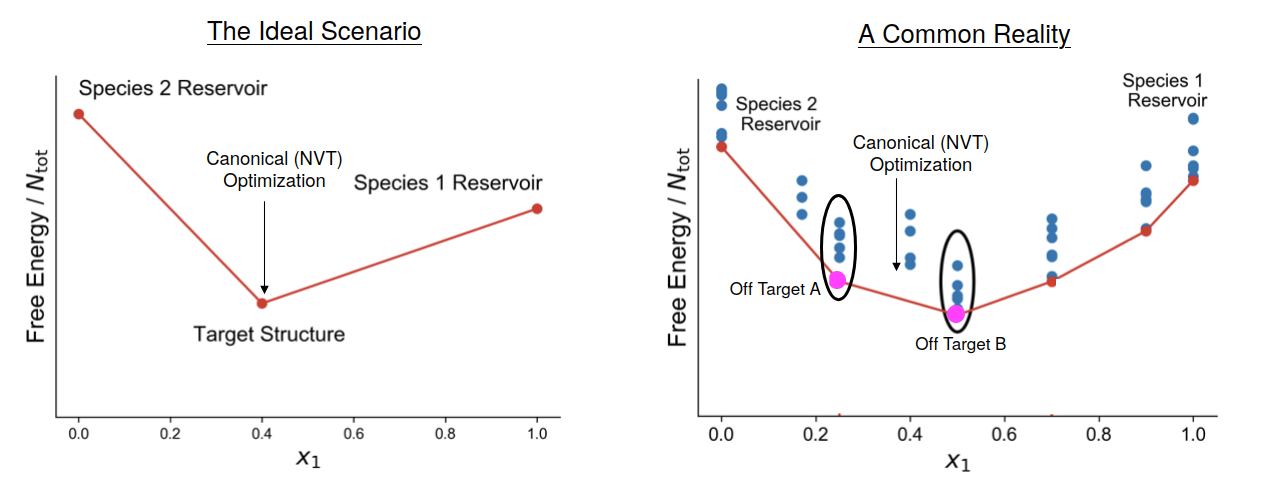
As a final note, observe that, in general, the phase diagrams do not contain only a single structure. In the "Ideal Scenario" cartoon above the target structure is the only one present in the "middle" of the hull. In other words, we have a reservoir of unassembled "A" particles and another reservoir of "B" particles (which are usually programmed not to assemble in the pure component state), and when mixed they form the target. If not mixed in the exact ratio, the leftover particles simple remain unassembled. But the "Common Reality" is exactly that. However, it is possible to view this as a feature instead of a "bug" in light of sensing applications. The particle chemistry or programming is fixed, so the only that causes the structural change is a concentration change, which could be observed along with the onset of another phenomenon we are trying to sense. It is possible to them imaging multiobjective versions of the optimization protocols mentioned above to build "switches" out of these systems.

Conclusions

Using symmetry we can devise methods to enumerate crystal structure ensembles that contain a diverse (all wallpaper groups) set of candidates. This enables a systematic search of crystalline configurations which can be used to do "forward" exploration, or "inverse" design when coupled with machine learning techniques. The algorithm we employed allows us to do this incredibly fast relative to the case where symmetry is not used to suppress the combinatorial explosion of possibilities. This relies on a convenient choice of how to generate the fundamental domain for each symmetry. This, however, is not unique. While that does not detract from the generality of our results, there are sometime other ways of making these choices which are convenient in other applications. This is the subject of ongoing work, as is the extension to consider anisotropic particles! There are also a variety of different routes that enable extensions to 3D Euclidean space, which are also under consideration.

zzz_basin_hopping.gif

zzz_gcid_example.gif