Science Fair

Fire_Science.md

Fire Science

Spatial Data Prerequisites

• Counties (polygons)
• Roads (polylines)
• Fires (points)
• Parks (polygons)

Exploratory Questions

• How many fires have occured within state parks and nearby state parks, aka 1 to 5 miles away?

• How many fires occured within .25 mile, .5 mile, 1 mile, 2 miles of a road?

• What is the human population density where the wildfire occured?

• What wildland urban interface have been subject to the most fires?

• What counties have the most fires?

Prepare data for analysis

Statewide spatial datasets have been collected from various authoritative sources.

Dataset	Source
Roads	USGS National Transportation Dataset (NTD) for California
Wildland Urban Interface	California Department of Forestry and Fire Protection's Fire and Resource Assessment Program (FRAP) (*)
County boundaries	California's Open Data Portal (*)
Wildfire ignition sites	United States Geological Survey (*)

*link attribution is incorrect. actual data provided by team members

Additional processing was done on the statewide datasets to organize fire ignitions, roads and WUI's by county. Two processes were used:

1. A field calc was done to replace spaces with underscores ( whitespace() script)
2. A clip analysis was done inside an iterative model to clip out data from each county boundary.

Once processing was complete 4 databases were created to support research efforts:

Fires.gdb

• Alameda_County_Fires
• Alpine_County_Fires
• Amador_County_Fires
• Butte_County_Fires ...

Roads.gdb

• Alameda_County_Roads
• Alpine_County_Roads
• Amador_County_Roads
• Butte_County_Roads ...

Wildlands.gdb

• Alameda_County_WUI
• Alpine_County_WUI
• Amador_County_WUI
• Butte_County_WUI ...

Parks.gdb

• Alameda_County_Parks
• Alpine_County_Parks
• Amador_County_Parks
• Butte_County_Parks ...

Issue to ponder

The fire science data originally came from 4 statewide data files. These files were then subdivided by county. What are the advantages and disadvantages of splitting a large statewide dataset into smaller county datasets? Might changing the shape and size of the data hide patterns, relationships and connections that may reveal underlying causes of wildfires? Will the analytical methods used to explore fire in one county be the same for another county?

Analytical methods

Use these methods to quantify your hypothesis and find answers to questions related to fire behavior.

Napa County Parkland analysis

1. Create a new map
2. Add Napa_County_Parks layer to the map
3. Click Analysis -> Buffer
4. Apply these Buffer tool values

Key	Value
Input Features	Parks.gdb\Napa_County_Parks
Output Feature Class	Parks.gdb\Napa_County_Parks_1_Miles
Linear Unit	use default setting
Distance	1 choose miles
Side Type	use default setting
Method	use default setting
Dissolve Type	use default setting

5. Run

Next repeate steps 1-5 again creating a 5 mile buffer. When done there will be 3 layers in the Content Pane. Toggle on and off the layers. Make a mental note that park boundries overlap with buffers applied.

Next perform a spatial join analysis using the park layers and wildfire ignition sites to obtain counts of fires in parks.

1. Add Napa_County_Fires layer to the map
2. Click Analysis -> Spatial Join
3. Apply these Spatial Join tool values

Key	Value
Target Features	Parks.gdb\Napa_County_Parks
Join Features	Fires.gdb\Napa_County_Fires
Output Feature Class	Parks.gdb\Napa_County_Parks_Fire_Cnt
Join Operation	use default setting
Keep All Target Features	use default setting
Field Map of Join Features	From bottom upward, delete all fields including GlobalID field using red x button
Match option	Completely contains

4. Run

Next repeate steps 1-4 again using the 1 mile and 5 mile park buffer layers.

When done right click on the Napa_County_Parks_Fire_Cnt layer in the Contents Pane. Then open the attribute table. The total number of fires for each park will be listed under the column named Join_Count.

Napa County Road analysis

Try using the above parks analysis, as your guide. The process should be the same but with different datasets, aka roads not parks and different buffer distances.

Napa County Human Population Density analysis

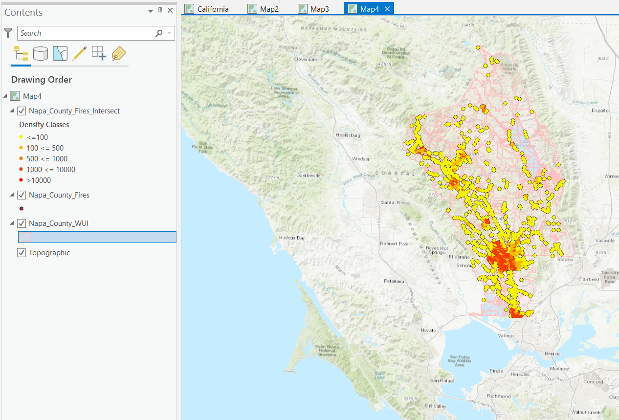
In order to explore fire incidents and human population density a missing demographic measure is needed. This measure needs to be assocated with each fire ignition point, but is actually assocated with each WUI boundary. One method to connect fire ignitions with WUI population densities might be SQL table joining. This might involve some form of primary and foreign key matching. However, in the case of spatial data we can use location to connect different layers of information together. Follow the next few step to see how location can be used to join layers of information together.

1. Create a new map
2. Add Napa_County_Fires layer to the map
3. Add Napa_County_WUI layer to the map
4. Click Analysis -> Intersect
5. Apply these Intersect tool values

Key	Value
Input Features	Fires.gdb\Napa_County_Fires (leave ranks empty)
Input Features	Wildlands.gdb\Napa_County_WUI (leave ranks empty)
Output Feature Class	Fires.gdb\Napa_County_Fires_Intersect
Attributes to Join	use default setting
XY Tolerance	use default setting
Output Type	use default setting

6. Run

When done right click on the Napa_County_Parks_Fires_Intersect layer in the Contents Pane. Then open the attribute table and observe the POPDEN2010 column alongside the wildfire ignition site data. Next right click on the layer again and select Symbology. From the symbology panel choose graduated color, select the field POPDEN2010, choose number of classes and pick a color ramp. The map should now illustrate wildfires according to population density.

Python scripts

def whitespace(fld):
    return fld.replace(" ", "_")
    

@aqitrade - Thanks for giving me access. I've uploaded the data. It's a total of 5 zips.

• Source.zip Source.gdb is a file geodatabase with your statewide files but with CA roads from USGS
• Fires.zip Fires.gdb is your allfires18_1 feature class organized by county in a file geodatabase
• Wildlands.zip Wildlands.gdb is your ca_wui_cp12 shapefile file organized by county in a file geodatabase
• Parks.zip Parks.gdb is your ParkBoundaries shapefile file organized by county in a file geodatabase
• Roads.zip Roads.gdb is statewide roads organized by county in a file geodatabase

Correct roads is a USGS National Transportation Dataset (NTD) for California.

Great tool tips on pop density analysis using join and symbology... I was able to follow the procedures. question: is there a way I can control how pop density are broken down by different classes? What’s the current mechanism behind the scene when I chose 5 classes, it breaks Pop density into <817.56, <2433.51, <4587.65, <8133.56, and <15929.88. Can I specify how I want to break pop density down, say <100, <500, <1000, <10000?

Additionally, I am trying to find out the count of fires in each pop density count range - there are a total of 4150 WUIs in Napa County, ranging from 0 to 15929.88. We are trying to determine, by County, the most number of fire occurrences in the same Pop Density range. Hence it’s important to custom define the fixed pop density range by ourselves.

I figured out how to make “Manual Interval” in the symbology... now trying to figure out the count in each range...

@aqitrade - Glad you were able to follow along on that one. In terms of controlling how pop density are broken down by different classes there are a few ways forward. When selecting Symbology and Graduated Color you can also click on the Upper Value for each class and manipulate class range values or you can take the Field Calculation approach.

For Field Calculation after computing the Intersect open the attribute table by right clicking on the Intersect layer. Once the table is open look for table icons at the top. Choose the one to Add a_New Field_. Name it something like Density_Classification. Then right click on the new column name and choose Calculate Field.

This opens up the Calculate Field tool. Because you right clicked on Density_Classification this will populate the entire empty column based on an expression you define. There are two really important tool parameters in the Calculate Field tool:

1. _Density_Classification =
2. Code Block

I usually start with code block and write a Python function that returns the desired value. Then I would fill out the single input next to the _Density_Classification =. It might look something like this:

Expression:
Reclass(!WELL_YIELD!)

Code Block:
def Reclass(WellYield):
    if (WellYield >= 0 and WellYield <= 10):
        return 1
    elif (WellYield > 10 and WellYield <= 20):
        return 2
    elif (WellYield > 20 and WellYield <= 30):
        return 3
    elif (WellYield > 30):
        return 4

Hopefully this approach makes sense. Calculate Field methods are very useful. Purposes can include weighting values and/or things like math and statistics operations like standard deviation. The resulting values then are typically used control layer symbology.

Further reading suggestions:

https://pro.arcgis.com/en/pro-app/tool-reference/data-management/calculate-field-examples.htm

https://pro.arcgis.com/en/pro-app/tool-reference/data-management/calculate-field.htm

Lastly on getting fire counts, after you reclassify, I believe you can use Summary Statistics which does things like SQL Group By and COUNT().

@aquitrade - Try Summary Statistics which does things like SQL Group By and COUNT(). Under Analysis the tool is in the Ribbon or you can search for this name after clicking Tools under Analysis.

Question on roads - the roads.gdb is a state wide database and are not broken down by counties right? Should we break the roads by County like the others?

@aqitrade The Roads.zip I believe contains Roads.gdb and in the file geodatabase are roads broken up county by county (like the other .gdb’s are organized). Is that not what you are seeing?

I must have messed up the file... now it is broken up by County as expected... thanks

Great. JFYI- after using the Summary Statistics tool it then possible to Join the result summarized table back to the Intersect table. Join is both a searchable tool and is also available as a context item when right clicking on the layer name, in the content pane.

I couldn’t figure out how to use summary statistics... there is no “sql group by” function. Count will only count the total number of rows... it seems like summary statistics only works on the entire Intersect table, not the symbolized layer by density classes...

@aqitrade Okay. Just to make sure I am tracking correctly. Intersect introduced WUI attributes (including POP DENSITY) into each fire. The task is now to know the total number of fires that occurred in each POP DENSITY class break range. Is that correct?

That is exactly right

Try this workflow. Following Intersect, right click on Napa_County_Fires_Intersect in the Content Pane. Open the Attribute Table. Next click Add Field icon in the table. Then name the new field DCLASSS_A and give it an Alias name of Density Classes A and assign a data type of LONG. Next click Save in the ribbon.

It might seem weird to classify using LONG (and not TEXT), but I think it may work better with graduated symbols.

Next review the attribute table of Napa_County_Fires_Intersect. Find the new field with alias name of Density Classes A and right click on it selecting Calculate Field.

Input the calculation code in the code block and call the ReClass() function passing in the POPDEN2010 field.

Expression:
Reclass(!POPDEN2010!)

Code block:
def Reclass(density):
    if (density >= 0 and density <= 100):
        return 1
    elif (density > 100 and density <= 500):
        return 2
    elif (density > 500 and density <= 1000):
        return 3
    elif (density > 1000 and density <= 10000):
        return 4
    elif (density > 10000):
        return 5

Once the density classifications have been persisted in the table, symbolize again using Graduated Color. Assign meaningful labels for each class and pick a color ramp that makes sense. As FYI - you can tweak each point symbol style properties (color, outline, etc) by clicking on the symbol.

Next to get the count of fires in each Density Class click Analysis in the Ribbon and then select the Summary Statistics tool. Apply these Summary Statistics tool values.

Key	Value
Input Table	Fires.gdb\Napa_County_Fires_Intersect
Output Table	Fires.gdb\Napa_County_Fires_Cnt_By_PopDen
Statistics Field	Density Classes A
Case field	Density Classes A

Then click, Run.

Everything works as instructed... very cool. I assume that I had to specify “statistic type” to be “count” for “statistic field” “density classes A” correct? If so I am doing the right thing.

I need a little help on how to style each symbol in the symbology... like color, shape, etc. where do I click to edit?

Lastly can you please upload the California topological map gdb to OneDrive? I like the background map layer you used.

@aqitrade - you are correct with that Stat type. My mistake. I missed that key and value. In terms of the topo map, on the ribbon there should be a button to switch out the basemap. It might be under the Map tab or Insert tab. The software include a variety of basemaps, topo being one of them.

Got it... I was also able to figure out the styling part... now the fun is on to run the data analysis :)

We tried different methods of pop density analysis and determined that standard deviation is a better way than hardcoding the intervals.

Now, the pop density is always a right screwed distribution so my goal is to identify by County the pop density boundary below which 80% of wildfires occurred. Then I will average all County numbers and use the pop density avg number as a threshold for those WUIs whose pop density are smaller, or higher likelihood to have wildfires.

Two questions: 1. How to calculate the pop density threshold of the WUIs that have 80% of wildfire occurrences?

2. The default histogram under symbology is not visually appealing - is there a way to export the underlying numbers to a table so that I can generate nicely looking histogram?

@aqitrade Regarding 1. would maybe suggest continued use of adding new fields/columns to tables and then using Calculate Field which supports math and comparison operators. Regarding 2. Yes you can export data. Here’s a link which explains that workflow.

https://pro.arcgis.com/en/pro-app/help/data/tables/export-tables.htm

Given that the majority of the fires occur within close distance of a road, how to find out how many fires occurred NOT within certain distance of a road (say 1 mile)? Which analysis tool can I use for that?

@aqitrade I would try intersecting your road buffer with the fires. Then for every fire that intersects with the buffer (with a fire) there should be a JoinCount value there. For each fire that does not intersect with the buffer there probably will be null values under the JoinCount field. Those are the ones you need to count. Summary Statistics tool could count these. Another technique would be to first create a field HasFire in the buffer layer and populate it with a 1 if JoinCount is greater than 0. Then do the intersection and count nulls in the HasFire column using Summary Statistics.

I just realized that the Fires.gbd you broke up into Counties include urban structure fires. The original IgnitionHistory18_1.gdb has two layers: one is allfires 18_1, the other is wildlandSRA18_1. For our project we are only studying wildland fires. Can you pls tell me how you can include only wildland fires into per County layer? There are only ~50k Wildland fires as opposed to ~720k fires in all fires gdb.

I might have to redo all the spatial intersections because I only want to use the wildland fire layer in the ignition gdb. Can you please help break it down into per County layers? Thanks so much.

Basically I want to break up the wildlandsra18_1 layer by Counties and save them into the new wildfires.gdb fire. Please let me know how to achieve that. Thanks

Oh gosh. My computer is at the office. I can get to this by end of day. Let me know, if you want me to take care of doing the clip. Essentially this is best accomplished via the Model Builder feature in the software. It’s a matter of adding a Feature Select iterator tool which is wired to the County Layer and County Name (aka Value) and then feed that into the Clip Tool which takes your Fires layer as an argument and the output of the Feature Iterator. Then the output of clip should go into a Fire Geodatabae with output name something like _MoreFires.gdb/%Value%_Fires2. (The value in % is the name of the County).

Let me know, as I could probably get this done by 5PM and uploaded to One Drive.

That will be awesome - thanks so much if you van do it today... we were about to do the conclusion this afternoon then realized the data analysis didn’t make sense for road proximity... then we realized it... lol... sorry if you have to run to office to do this work for the girls... it will be so helpful thank you again

@aqitrade ok that works. Not a problem. Will let you know when it’s done.

@aqitrade I've uploaded a new zip named Wildlandsra18_1 that contains Wildlandsra18_1.gdb with wildlandsra18_1 layers organized by county. It's in the One Drive.

Cool thakst

One of the issues we ran into is during buffer analysis we may have the same fires spatially joining multiple polygons so that duplicates are counted in the total Joint_Count of all parks. This is especially a problem for park analysis as some park buffers (e.g. 3 mile buffer) are overlapping with each other. As such we want to figure out all the fires that are NOT in any park/park buffer polygons instead. What analysis tool should we use for that?

Simply put, how many points are not in the set of polygons?

Ok I figured out a way - first merge all the ploygons in the same layer that have overlaps into a single big polygon then do spatial join with the fires... this is fun