README.md

This is a proof-of-concept of how an R Markdown Notebook can be converted into an IPython Notebook. The idea is to allow R users to author reproducible documents in R Markdown, but be able to seamlessly convert into HTML or an IPython Notebook, which allows greater interactivity.

The bulk of the work here is done by notedown, a python module that helps create IPython notebooks from markdown. The approach I have taken here is to convert the RMarkdown file into a Markdown file using a custom knitr script, and then using notedown to render it as an IPython notebook.

If you want to test it out, install the notedown module and run make example.ipynb.

You can view the converted IPython Notebook on nbviewer

example.Rmd

## Introduction to ggplot2

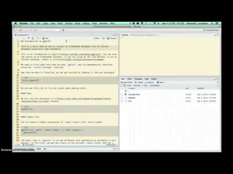
This is a short demo on how to convert an R Markdown Notebook into an IPython Notebook using knitr and notedown.

Adding a Python Chunk

```{r engine="python"}
def f(x):
  return x + 2
f(2)
```

This is an introduction to [ggplot2](http://github.com/hadley/ggplot2). You can view the source as an R Markdown document, if you are using an IDE like RStudio, or as an IPython notebook, thanks to [notedown](https://github.com/aaren/notedown).

We need to first make sure that we have `ggplot2` and its dependencies installed, using the `install.packages` function.

Now that we have it installed, we can get started by loading it into our workspace

```{r}
library(ggplot2)
```

We are now fully set to try and create some amazing plots. 

#### Data

We will use the ubiqutous [iris](http://stat.ethz.ch/R-manual/R-patched/library/datasets/html/iris.html) dataset.

```{r}
head(iris)
```

#### Simple Plot

Let us create a simple scatterplot of `Sepal.Length` with `Petal.Length`.

```{r}
ggplot(iris, aes(x = Sepal.Length, y = Petal.Length)) +
  geom_point()
```

The basic idea in `ggplot2` is to map different plot aesthetics to variables in the dataset. In this plot, we map the x-axis to the variable `Sepal.Length` and the y-axis to the variable `Petal.Length`.

#### Add Color

Now suppose, we want to color the points based on the `Species`. `ggplot2` makes it really easy, since all you need to do is map the aesthetic `color` to the variable `Species`.

```{r}
ggplot(iris, aes(x = Sepal.Length, y = Petal.Length)) +
  geom_point(aes(color = Species))
```

Note that I could have included the color mapping right inside the `ggplot` line, in which case this mapping would have been applicable globally through all layers. If that doesn't make any sense to you right now, don't worry, as we will get there by the end of this tutorial.

#### Add Line

We are interested in the relationship between `Petal.Length` and `Sepal.Length`. So, let us fit a regression line through the scatterplot. Now, before you start thinking you need to run a `lm` command and gather the predictions using `predict`, I will ask you to stop right there and read the next line of code.

```{r}
ggplot(iris, aes(x = Sepal.Length, y = Petal.Length)) +
  geom_point() + 
  geom_smooth(method = 'lm', se = F)
```

If you are like me when the first time I ran this, you might be thinking this is voodoo! I thought so too, but apparently it is not. It is the beauty of `ggplot2` and the underlying notion of grammar of graphics.

You can extend this idea further and have a regression line plotted for each `Species`.

```{r}
ggplot(iris, aes(x = Sepal.Length, y = Petal.Length, color = Species)) +
  geom_point() + 
  geom_smooth(method = 'lm', se = F)
```

knit

#!/usr/bin/Rscript

library(knitr)
opts_chunk$set(eval = FALSE)
rmd = paste("```\n%load_ext rmagic\n```\n\n", 
  paste(readLines('example.Rmd'), collapse = '\n'),
  collapse = '\n'
)
knit(text = rmd, output = 'example.md')

Makefile

example.md: example.Rmd
	Rscript ./knit

example.ipynb: example.md
	c://python27_64/scripts/notedown example.md | sed 's/%%r/%%R/' > example.ipynb