A simple comparison of two models with different feature set approaches

lm_vs_nnet.R

library(tidymodels)
library(doMC)

# ------------------------------------------------------------------------------

tidymodels_prefer()
theme_set(theme_bw())
options(pillar.advice = FALSE, pillar.min_title_chars = Inf)
registerDoMC(cores = parallel::detectCores())

# ------------------------------------------------------------------------------

data("Chicago")

n <- nrow(Chicago)
p <- 1 - (14/n)

Chicago <- 
  Chicago %>% 
  select(ridership, date)

init_split <- initial_time_split(Chicago, prop = p)
chi_train <- training(init_split)
chi_test <- testing(init_split)

# ------------------------------------------------------------------------------
# The effects in the data are almost completely driven by the day-of-the-week 
# and holidays. For example:

plot_start <- 1050
chi_train %>% 
  mutate(
    day = lubridate::wday(date, label = TRUE),
    day = factor(day, ordered = FALSE)
  ) %>% 
  slice(plot_start:(plot_start + 35)) %>% 
  ggplot(aes(date, ridership)) +
  geom_point(aes(col = day), cex = 2) + 
  geom_line(alpha = .2)

# ------------------------------------------------------------------------------

chi_rs <-
  chi_train %>%
  sliding_period(
    index = c(date),  
    period = "week",
    lookback = 12 * 52,
    assess_stop = 2,
    step = 2 
  )

# ------------------------------------------------------------------------------
# Use a handful of date features to get good preformance

lm_rec <- 
  recipe(ridership ~ date, data = chi_train) %>% 
  step_date(date) %>% 
  step_holiday(date) %>% 
  update_role(date, new_role = "date id")

lm_res <- 
  linear_reg() %>% 
  fit_resamples(lm_rec, chi_rs)

collect_metrics(lm_res)

# ------------------------------------------------------------------------------
# Convert data to integers and let the network figure it out. 

nnet_rec <- 
  recipe(ridership ~ date, data = chi_train) %>% 
  step_mutate(day_index = as.numeric(date)) %>% 
  step_normalize(day_index) %>% 
  update_role(date, new_role = "date id")

nnet_spec <- 
  mlp(
    hidden_units = tune(),
    penalty = tune(),
    epochs = tune()
  ) %>%
  set_mode("regression") %>% 
  # open up the range of the initial values ('rang') in case that's an issue
  set_engine("nnet", rang = 0.75)

print(translate(nnet_spec))

nnet_param <- 
  nnet_spec %>% 
  extract_parameter_set_dials() %>% 
  update(
    hidden_units = hidden_units(c(2, 100)),
    epochs = epochs(c(150, 10000))
    )

set.seed(3828)
nnet_res <- 
  nnet_spec %>% 
  tune_grid(nnet_rec, chi_rs, grid = 25, param_info = nnet_param)

show_best(nnet_res)
autoplot(nnet_res)

nnet_fit <- 
  workflow(
    nnet_rec,
  finalize_model(nnet_spec, select_best(nnet_res, metric = "rmse"))
  ) %>% 
  fit(chi_train)

augment(nnet_fit, chi_train) %>% 
  mutate(
    day = lubridate::wday(date, label = TRUE),
    day = factor(day, ordered = FALSE)
  ) %>% 
  slice(plot_start:(plot_start + 35)) %>% 
  ggplot(aes(day_index, ridership)) +
  geom_point(aes(col = day), cex = 2) + 
  geom_line(aes(y = .pred))

# ------------------------------------------------------------------------------
# Use the simple features with the network

nnet_feat_rec <- 
  recipe(ridership ~ date, data = chi_train) %>% 
  step_mutate(day_index = as.numeric(date)) %>% 
  step_date(date) %>% 
  step_holiday(date) %>% 
  update_role(date, new_role = "date id") %>% 
  step_range(all_numeric_predictors()) %>% 
  step_dummy(all_factor_predictors(), one_hot = TRUE)

set.seed(3828)
nnet_feat_res <- 
  nnet_spec %>% 
  tune_grid(nnet_feat_rec, chi_rs, grid = 25, param_info = nnet_param)

autoplot(nnet_feat_res)

Hey Max,
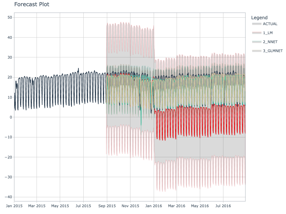
I played around with lm, nnet, and glmnet just to give you some quick insights. I'll summarize the insights below, and then give you the code to reproduce.

Insights

My approach differs a bit:

1. I want to add a lot of features off the bat to give the models as much information as possible. For models like LM, they tend to overfit because of this.
2. When using Machine Learning, an advantage is the penalty parameter. NNET and GLMNET have this to help with feature selection and penalizing poor features.

What I see is that LM overfits badly with the features I gave it. NNET and GLMNET do well.

The future forecast looks much better with the GLMNET model as compared to the NNET model. This is because I did not perform tuning. But it's worth noting that the GLMNET is very simple - Just add a little penalty and it needs no tuning to give a good forecast. NNET needs tuning.

Code

library(tidymodels)
library(timetk)
library(modeltime)

chicago_tbl <- Chicago %>%
    select(date, ridership)

chicago_tbl %>%
    plot_time_series(date, ridership)

# TRAIN/TEST SPLIT ----

splits <- time_series_split(chicago_tbl, assess = "1 year", initial = "5 year")

splits %>%
    tk_time_series_cv_plan() %>%
    plot_time_series_cv_plan(date, ridership)

# MODELING ----

rec_lm <- recipe(ridership ~ date, data = training(splits)) %>%
    step_timeseries_signature(date) %>%
    step_rm(date) %>%
    step_zv(all_numeric_predictors()) %>%
    step_normalize(all_numeric_predictors()) %>%
    step_dummy(all_nominal_predictors(), one_hot = FALSE)
    

rec_lm %>% prep() %>% bake(training(splits)) %>% glimpse()

# * Linear Regression lm ----

wflw_lm <- workflow() %>%
    add_model(linear_reg() %>% set_engine("lm")) %>%
    add_recipe(rec_lm) 

wflw_lm_fit <- wflw_lm %>% fit(training(splits))

# * Neural Net nnet ---- 

wflw_mlp <- workflow() %>%
    add_model(mlp("regression") %>% set_engine("nnet")) %>%
    add_recipe(rec_lm)

wflw_mlp_fit <- wflw_mlp %>% fit(training(splits))

# * Elastic Net glmnet -----

wflw_glmnet <- workflow() %>%
    add_model(linear_reg(penalty = 0.01) %>% set_engine("glmnet")) %>%
    add_recipe(rec_lm) 

wflw_glmnet_fit <- wflw_glmnet %>% fit(training(splits))

# MODEL COMPARISON ----

model_tbl <- modeltime_table(
    wflw_lm_fit,
    wflw_mlp_fit, 
    wflw_glmnet_fit
)

calib_tbl <- model_tbl %>% modeltime_calibrate(testing(splits))

calib_tbl %>% modeltime_accuracy()

test_forecast_tbl <- calib_tbl %>%
    modeltime_forecast(
        new_data = testing(splits),
        actual_data = chicago_tbl
    ) 

test_forecast_tbl %>%
    filter_by_time(.start_date = "2015") %>%
    plot_modeltime_forecast()

# FUTURE FORECAST ----

refit_tbl <- calib_tbl %>%
    modeltime_refit(
        data = chicago_tbl
    )

future_tbl <- chicago_tbl %>%
    future_frame(date, .length_out = 365)
    
future_forecast_tbl <- refit_tbl %>%
    modeltime_forecast(
        new_data = future_tbl, 
        actual_data = chicago_tbl
    )

future_forecast_tbl %>%
    filter_by_time(.start_date = "2015") %>%
    plot_modeltime_forecast()