Conformal prediction for linear regression and random forest. NB: pretty ugly and slow code.

conformal.R

# conformal prediction intervals for linear regression and random forest
library(tidyverse)
library(pbapply)
library(parallel)

# fully conformal prediction
conformal_quantile <- function(x, y, x_new, y_new, frm) {
  N <- length(x)
  df <- tibble(x = c(x, x_new), y = c(y, y_new))
  fy <- lm(frm, df)
  scores <- residuals(fy)^2
  # find the quantile of y_new score
  return(ecdf(scores[1:N])(scores[N+1]))
}

conformal_interval <- function(x, y, x_new, frm, level = 0.95, resolution = 0.1, min_y = mean(x) - IQR(x)*3, max_y = mean(x) + IQR(x)*3) {
  y_new <- seq(min_y, max_y, resolution)
  y_qtl <- vapply(y_new, conformal_quantile, x = x, y = y, x_new = x_new, frm = frm, FUN.VALUE = 0.)
  out <- if (all(y_qtl >= level)) c(-Inf, Inf) else range(y_new[y_qtl < level])
  names(out) <- c("lwr", "upr")
  return(out)
}



# tryout
set.seed(456)
N <- 1000
x <- rnorm(N) + 2
f <- function(x) 1+x-2*x^2+0.3*x^3
y <- f(x) + rnorm(N)


plot(x, y)
df <- tibble(x = x, y = y)
frm <- y ~ poly(x, 3)
fit <- lm(frm, df)


x_new <- seq(min(x) - 0.1, max(x) + 0.1, 0.1)
pred <- predict(fit, data.frame(x = x_new), interval = "pred", level = 0.95)
conf <- t(pbsapply(x_new, conformal_interval, x = x, y = y, min_y = -23, max_y = 9, res = 0.1, frm = frm))
colnames(conf) <- c("lwr_c", "upr_c")
as_tibble(pred) |> 
  bind_cols(conf) |> 
  mutate(x = x_new) |> 
  ggplot(aes(x = x, y = fit)) +
  geom_ribbon(aes(ymin = lwr, ymax = upr), fill = "#ababab") +
  geom_ribbon(aes(ymin = lwr_c, ymax = upr_c), fill = "#ab12ab") +
  geom_line() +
  geom_point(data = tibble(x = x, fit = y))
  


# tryout with ranger
conformal_quantile_rf <- function(x, y, x_new, y_new, frm) {
  N <- length(x)
  df <- tibble(x = c(x, x_new), y = c(y, y_new))
  fy <- ranger(frm, df)
  scores <- (df$y - predict(fy, df)$predictions)^2
  # find the quantile of y_new score
  return(ecdf(scores[1:N])(scores[N+1]))
}

conformal_interval_rf <- function(x, y, x_new, frm, level = 0.95, resolution = 0.1, min_y = mean(x) - IQR(x)*3, max_y = mean(x) + IQR(x)*3) {
  y_new <- seq(min_y, max_y, resolution)
  y_qtl <- vapply(y_new, conformal_quantile_rf, x = x, y = y, x_new = x_new, frm = frm, FUN.VALUE = 0.)
  out <- if (all(y_qtl >= level)) c(-Inf, Inf) else range(y_new[y_qtl < level])
  names(out) <- c("lwr", "upr")
  return(out)
}

frm <- y ~ x
fit <- ranger(frm, df)



x_new <- seq(min(x) - 0.1, max(x) + 0.1, 0.1)
pred <- predict(fit, data.frame(x = x_new))$prediction

cl <- makeCluster(10)
clusterExport(cl, c("conformal_interval_rf", "conformal_quantile_rf", "x", "y", "frm"))
clusterEvalQ(cl, {
  library(ranger)
  library(tibble)
})

conf <- pbsapply(x_new,
  function(xn) conformal_interval_rf(
    x          = x,
    y          = y,
    x_new      = xn,
    frm        = frm,
    resolution = 0.1,
    min_y      = -23,
    max_y      = 9
  ),
  cl = cl
)

stopCluster(cl)
rownames(conf) <- c("lwr_c", "upr_c")
tibble(fit = pred) |> 
  bind_cols(t(conf)) |> 
  mutate(x = x_new, lwr_c = smooth(lwr_c), upr_c = smooth(upr_c)) |> 
  ggplot(aes(x = x, y = fit)) +
  geom_ribbon(aes(ymin = lwr_c, ymax = upr_c), fill = "#ab12ab") +
  geom_line() +
  geom_point(data = tibble(x = x, fit = y))

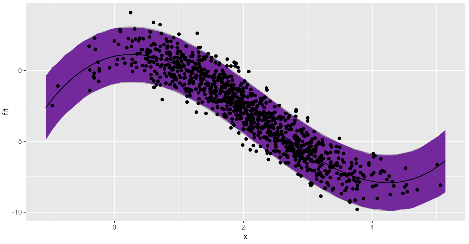
Linear regression prediction interval looks a lot like the standard interval, which is good because data were generated and modeled with all the correct assumptions:

Random forest smoothed prediction interval is computationally very intensive, but possible! See here: