Hello student,
Well done in your first submission! 👏 👏 A few minor changes are still required in order to meet our rubric. Keep doing this great job!
Cheers,
Student's implementation correctly calculates the following:
- Number of records
- Number of individuals with income >$50,000
- Number of individuals with income <=$50,000
- Percentage of individuals with income > $50,000
No big deal here. Kindly note that greater_percent is a percentage, not a decimal value. Are you sure that the graduation rate is 0.25%?
Student correctly implements one-hot encoding for the feature and income data.
Well done using the map method combined with a lambda function!
This reference provides 7 different encoding strategies. Binary encoding is a great choice for cases where the number of categories for a given feature is very high. Lately, entity embedding has increasingly becoming a very popular choice as well. Another of my favorite personal choices is to train models using LightGBM. It can handle categorical features without the need of one-hot encoding them.
Student correctly calculates the benchmark score of the naive predictor for both accuracy and F1 scores.
Great job calculating the accuracy and the F-score for a Naive predictor!
Note that the F-score is higher than the accuracy which seems counter-intuitive since the F-score is a more elaborate calculation. That happens because a value of beta = 0.5 attenuates the influence of false negatives. In other words, this value of beta weights more the positive predictions (>50K) than the negative one (<=50K).
The pros and cons or application for each model is provided with reasonable justification why each model was chosen to be explored. Please list all the references you use while listing out your pros and cons.
Please make it clear in your answer for each estimator the application, advantage, weakness and why it is a good candidate. For example, for adaboost, it is unclear whether the following sentence is an advantage or a reason to be a good candidate:
The reason it works well is because it takes "week classifiers" (such as decision trees) and combine their result to improve to a "strong classifier"
For listing their advantages and disadvantages, I highly suggest using sklearn documentation. I couldn't find for AdaBoost, but for other estimators like SGD it is possible to find.
Student successfully implements a pipeline in code that will train and predict on the supervised learning algorithm given.
Everything looks great here!
Student correctly implements three supervised learning models and produces a performance visualization.
As described in the project:
- Use a 'random_state' for each model you use, if provided.
Please make sure to use a random_state for each estimator (if available) in order to guarantee the reproducibility of your results.
Justification is provided for which model appears to be the best to use given computational cost, model performance, and the characteristics of the data.
I agree with your choice of AdaBoost! It is one of the best estimators for this project and in the analysis is the one which is leading to the highest test score. In general, tree-based estimators do better in this project because they have the flexibility to create non-linear decision boundaries, thus opening space for greater generalisation potential after tuning.
Student is able to clearly and concisely describe how the optimal model works in layman's terms to someone who is not familiar with machine learning nor has a technical background.
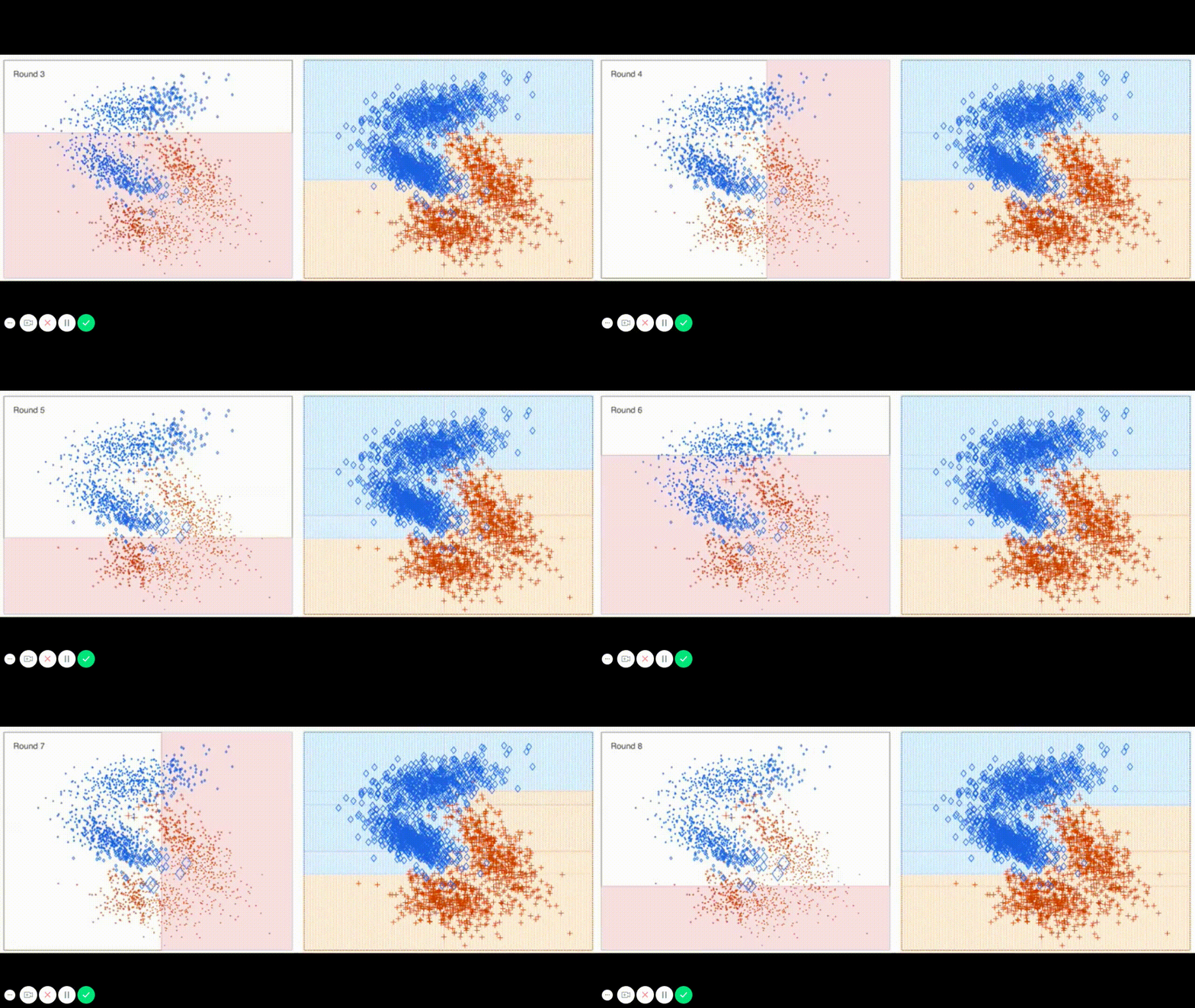
This video shows AdaBoost in action. It might be useful to get an intuition of how this estimator works. I suggest that you watch it in slow motion:
The final model chosen is correctly tuned using grid search with at least one parameter using at least three settings. If the model does not need any parameter tuning it is explicitly stated with reasonable justification.
Likewise before, please make sure to also set a random_state to the classifier here.
Student reports the accuracy and F1 score of the optimized, unoptimized, models correctly in the table provided. Student compares the final model results to previous results obtained.
Great job! Scores higher than 0.74 are only accomplished with boosting algorithms in this project! The best score I've seen was with Gradient Boosting (0.75).
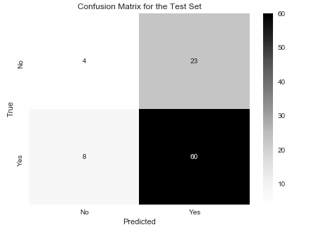
You can also check your results with a Confusion Matrix:
import seaborn as sns # Install using 'pip install seaborn'
from sklearn.metrics import confusion_matrix
import matplotlib.pyplot as plt
%matplotlib inline

cm_test = confusion_matrix(y_test, best_clf.predict(X_test))

plt.figure(figsize=(7,5))
sns.heatmap(cm_test, annot=True, cmap='Greys', xticklabels=['No', 'Yes'], yticklabels=['No', 'Yes'])
plt.title('Confusion Matrix for the Test Set')
plt.ylabel('True')
plt.xlabel('Predicted')
Student ranks five features which they believe to be the most relevant for predicting an individual's’ income. Discussion is provided for why these features were chosen.
Although it is a minor change, please make sure to also include a discussion on why the features were chosen. As mentioned in the question:
- and in what order would you rank them and why?
Student correctly implements a supervised learning model that makes use of the feature_importances_ attribute. Additionally, student discusses the differences or similarities between the features they considered relevant and the reported relevant features.
It is worth noting that each model with feature_importances_ might return different top predictive features depending on their internal algorithm implementation.
You can also use the attribute feature_importances_ from best_clf since it is already tuned so you will have a better choice of top 5 features:
importances = best_clf.feature_importances_
Student analyzes the final model's performance when only the top 5 features are used and compares this performance to the optimized model from Question 5.
An alternative strategy for reducing the number of features is to use dimensionality reduction techniques (PCA for example). Then, we could pick only the top descriptive features for training the model. You will see more details about PCA in the next module.

