Calculate the ratiation model in R

radiation_model.R

#' Code by Rafael H. M. Pereira and Marcus Saraiva
#'
#' Radiation model (Simini et al 2012)
#' Tij = Ti * ((Pi * Pj) / ((Pi + Pij) * (Pi + Pj + Pij)))
#' 
#' Where:
#'
#' Tij: Avarage flux between origin i and destination j predicted by the radiation model
#' Ti:  Proportion of population in i relative to total population
#' Pi:  Absolute population in i
#' Pj:  Absolute population in j
#' Pij: Absolute population potentially reacheable from i under the travel 
#'      necessary to tavel between i and j, excluding the population in i and j 
#'
#' Reference:
#'  Simini, F., González, M. C., Maritan, A., & Barabási, A. L. (2012). A universal
#'  model for mobility and migration patterns. Nature, 484(7392), 96-100.
#'

### load libraries --------------------------------------------------------
library(r5r)
library(ggplot2)
library(dplyr)
library(data.table)
library(pbapply)
library(furrr)
library(future)
library(ggpointdensity)
library(viridisLite)

options(scipen = 999)


### calculate travel tim matrix   --------------------------------------------------------

# build transport network
data_path <- system.file("extdata/poa", package = "r5r")
r5r_core <- setup_r5(data_path = data_path, temp_dir = TRUE)

# load origin/destination points 
points <- read.csv(file.path(data_path, "poa_hexgrid.csv"))

# keep only points with population
points <- subset(points, population  > 0)

# calculate travel time matrix
tt <- travel_time_matrix(r5r_core,
                         origins = points,
                         destinations = points,
                         mode = "WALK",
                         max_trip_duration = 200)


head(points)
head(tt)

### calculate components of the radiation model  --------------------------------------------------------

tt[points, on=c('fromId'='id'), pop_orig := i.population ]
tt[points, on=c('toId'='id'),   pop_dest := i.population ]

head(tt)
tail(tt)

# total population
pop_total <- sum(points$population)

# Share of total population in each origin 
tt[, Ti := pop_orig / pop_total, by = fromId]


# total pop_orig accessible from origin give max the travel time between o-d pair
# excluding the pop in O and D

# part 1

# get unique combinations of origin and travel time
a <- tt[,  .(fromId, travel_time )]
a <- unique(a)
a[, row := .I]

part1_fun <- function(i, ...){ # i = 50000
  
  orig <- a$fromId[i]
  tlimit <- a$travel_time[i]
  temp <- setDT(tt)[ fromId==orig, .(pij_part1 = sum(pop_dest[which(travel_time <= tlimit)])), by= fromId ]
  temp$travel_time <- tlimit
  return(temp)
}

future::plan(strategy = 'multisession')
part1_output <- furrr::future_map(.x = a$row, .f = part1_fun, .progress = TRUE)
part1_output <- rbindlist(part1_output)
# part1_output <- pblapply(X= a$row, FUN = part1_fun)

head(part1_output)

# merge
tt[part1_output, on=c('fromId', 'travel_time'), pij_part1  := i.pij_part1 ]
tt[, pij_part1 := fifelse(is.na(pij_part1), 0, pij_part1)]
head(tt)

# part 2
tt[, pij_part2 := pij_part1 - pop_dest, by=.(fromId, toId)]


### calculate radiation model  --------------------------------------------------------

tt[, rad := Ti * ((pop_orig * pop_dest) / ((pop_orig + pij_part2) * (pop_orig + pop_dest + pij_part2))), by=.(fromId, toId)]
summary(tt$rad)



### check results  --------------------------------------------------------

# remove Inf values
df <- subset(tt, rad < Inf)
summary(df$rad)
summary(df$travel_time)

plot( density(df$travel_time) )
plot( density(df$rad) )



# plot a sample of the results
sample_size <- 0.10
draw <- sample(x = 1:nrow(df), size = sample_size * nrow(df), replace = F)
df2 <- df[draw,]

ggplot() + 
  geom_density(data=df2, aes(x=travel_time, weight=rad), alpha=.1)


ggplot() + 
  geom_pointdensity(data=df2, aes(x=travel_time , y=rad), alpha=.1) +
  scale_color_viridis_c() +
  scale_y_log10()

I've mapped some flows, and it looks like people are not very interested in working far from home:

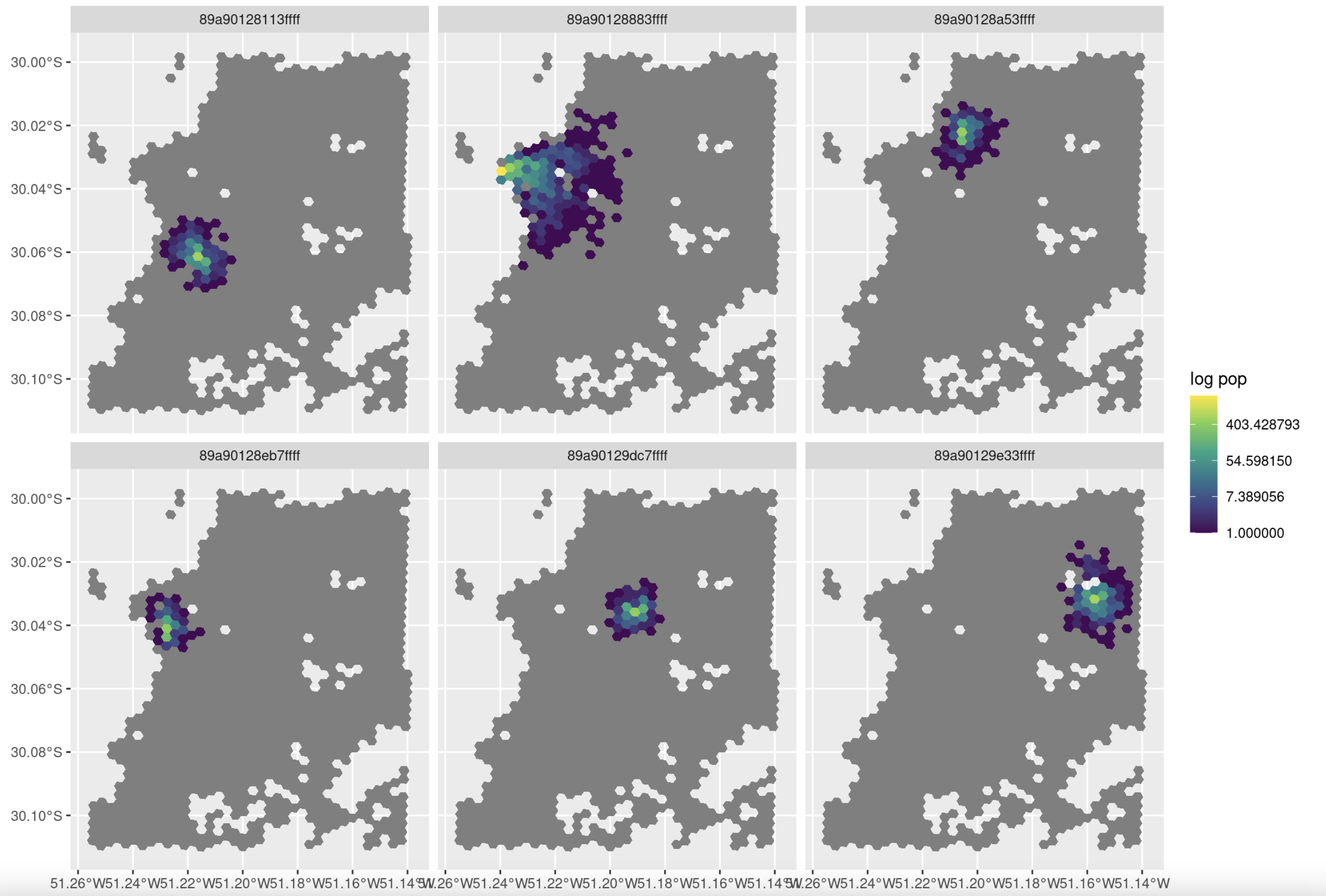
Code:

# Map results
library(h3jsr)
library(sf)

tt[, rad_pop := round(rad * pop_total)]
p_hex <- h3jsr::h3_to_polygon(points$id, simple = FALSE)

s_origins = sample(points$id, size = 6, prob = points$population)

df3 <- tt[fromId %in% s_origins & rad_pop > 0]
df3$geometry <- h3jsr::h3_to_polygon(df3$toId)
df3 <- st_as_sf(df3, crs = 4326)

ggplot(df3) +
  geom_sf(data = p_hex, fill = "grey50", color = NA) +
  geom_sf(aes(fill = rad_pop), color = NA) +
  facet_wrap(~fromId) +
  scale_fill_viridis_c(trans = "log") +
  labs(fill = "log pop")

thanks, Marcus! I've updated the code to incorporate the corrections you suggested !