how to create a world map using full hemispheric orthographic projection in `R`

ortho_map.md

Simple example of how to create a world map using full hemispheric orthographic projection in R

library(sf)
library(ggplot2)
library(mapview)
library(lwgeom)
library(rnaturalearth)
library(dplyr)

# world data
world <- rnaturalearth::ne_countries(scale = 'small', returnclass = 'sf')


# Fix polygons so they don't get cut in ortho projection
world  <- st_cast(world, 'MULTILINESTRING') %>%
  st_cast('LINESTRING', do_split=TRUE) %>%
  mutate(npts = npts(geometry, by_feature = TRUE)) %>%
  st_cast('POLYGON')

# map
ggplot() +
  geom_sf(data=world, color="gray80", aes(fill=continent)) +
  coord_sf( crs= "+proj=ortho +lat_0=20 +lon_0=-30")

ggplot() +
  geom_sf(data=world, color="gray80", aes(fill=continent)) +
  coord_sf( crs= "+proj=ortho +lat_0=20 +lon_0=90")

ortho_map2.md

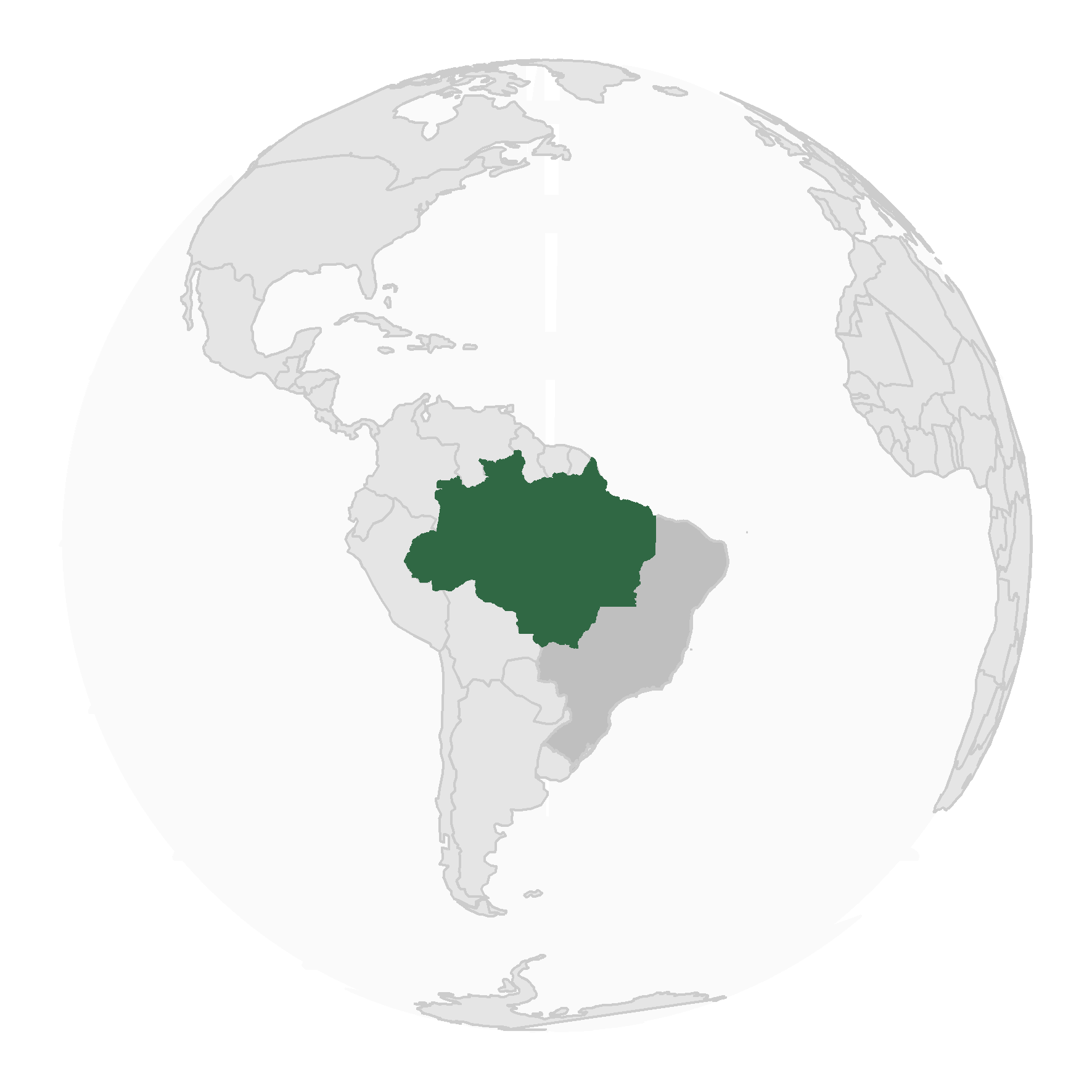
Simple way to create a map showing Brazil's Legal Amazon

# Libraries
library(geobr)
library(sf)
library(dplyr)
library(mapview)
library(lwgeom)
library(ggplot2)
library(rnaturalearth)
library(ggthemes)



### Brazil map ------------------------------------

amazon <- geobr::read_amazon()
brazil <- geobr::read_country()



### World map ------------------------------------
world <- rnaturalearth::ne_countries(scale = 'small', returnclass = 'sf')

  # Fix polygons to ortho projection, following from @fzenoni: https://github.com/r-spatial/sf/issues/1050
  world  <- st_cast(world, 'MULTILINESTRING') %>%
                    st_cast('LINESTRING', do_split=TRUE) %>%
                    mutate(npts = npts(geometry, by_feature = TRUE)) %>%
                    st_cast('POLYGON')


# Define the orthographic projection
  # Choose lat_0 with -90 <= lat_0 <= 90 and lon_0 with -180 <= lon_0 <= 180
  lat <- -6
  lon <- -57
  ortho <- paste0('+proj=ortho +lat_0=', lat, ' +lon_0=', lon, ' +x_0=0 +y_0=0 +a=6371000 +b=6371000 +units=m +no_defs')


# globe border
  globe <- st_graticule(ndiscr = 10000, margin = 10e-6) %>%
    st_transform(crs = ortho) %>%
    st_convex_hull() %>%
    summarise(geometry = st_union(geometry))  




### Plot  ------------------------------------

temp_plot <- ggplot() +
              geom_sf(data=globe, fill="gray98", color="gray98") +
              geom_sf(data=world, fill="gray90", color="gray80") +
              geom_sf(data=brazil, fill="gray75", color="gray80") +
              geom_sf(data=amazon, fill="#306844", color="#306844") +
              theme_map()
  
  
              ## zoom
              # + coord_sf(datum =ortho, xlim = c(st_bbox(brazil2)[[1]], st_bbox(brazil2)[[3]]), ylim = c(st_bbox(brazil2)[[2]], st_bbox(brazil2)[[4]]), expand = FALSE) 
              # brazil2 <- st_transform(brazil, crs = ortho)

# save plot
ggsave(temp_plot, file='geobr_brazilian_amazon_legal.png', dpi = 300, width = 15, height = 15, units = "cm", bg = "transparent")

Another example, with fixed topologies