Choropleth using an external geojson (DC Census Tracts by Population Change - 2000), data-driven styling, and queryRenderedFeatures to show hovered polygon's features in a sidebar tooltip.
Kyle Walker walkerke
etachov
/ nyt_style_buildings.R
Created
October 14, 2018 16:23
Making NYT-style building maps with data from Microsoft
This file contains hidden or bidirectional Unicode text that may be interpreted or compiled differently than what appears below. To review, open the file in an editor that reveals hidden Unicode characters.
Learn more about bidirectional Unicode characters
| library(tidyverse) | |
| library(sf) | |
| library(tigris) | |
| # start by picking a state from https://github.com/Microsoft/USBuildingFootprints | |
| # WARNING: these files can be pretty big. using arizona for its copious subdivisions and reasoanable 83MB. | |
| url_footprint <- "https://usbuildingdata.blob.core.windows.net/usbuildings-v1-1/Arizona.zip" | |
| download.file(url_footprint, "Arizona.zip") | |
| unzip("Arizona.zip") |
This file contains hidden or bidirectional Unicode text that may be interpreted or compiled differently than what appears below. To review, open the file in an editor that reveals hidden Unicode characters.
Learn more about bidirectional Unicode characters
| <!DOCTYPE html> | |
| <html> | |
| <head> | |
| <meta charset='utf-8' /> | |
| <title></title> | |
| <link href='https://api.tiles.mapbox.com/mapbox-gl-js/v0.26.0/mapbox-gl.css' rel='stylesheet' /> | |
| <link href='https://www.mapbox.com/base/latest/base.css' rel='stylesheet' /> | |
| <link href='site.css' rel='stylesheet' /> | |
| </head> | |
| <body class='clip loading'> |
ndrhzn
/ population_pyramid.R
Created
May 22, 2016 18:04
This file contains hidden or bidirectional Unicode text that may be interpreted or compiled differently than what appears below. To review, open the file in an editor that reveals hidden Unicode characters.
Learn more about bidirectional Unicode characters
| library(magrittr) | |
| library(dplyr) | |
| library(ggplot2) | |
| population <- read.csv("https://raw.githubusercontent.com/andriy-gazin/datasets/master/ageSexDistribution.csv") | |
| population %<>% | |
| tidyr::gather(sex, number, -year, - ageGroup) %>% | |
| mutate(ageGroup = gsub("100 і старше", "≥100", ageGroup), | |
| ageGroup = factor(ageGroup, |
hrbrmstr
/ acsdownforeveryoneorjustme.r
Created
March 26, 2016 18:54
This file contains hidden or bidirectional Unicode text that may be interpreted or compiled differently than what appears below. To review, open the file in an editor that reveals hidden Unicode characters.
Learn more about bidirectional Unicode characters
| purrr::map_df(2009:2014, function(i) { | |
| api_info <- jsonlite::fromJSON(sprintf("http://api.census.gov/data/%s/acs5/", i)) | |
| api_info$dataset[, c("title", "c_unavailableMessage")] | |
| }) |
hrbrmstr
/ ahealth.md
Last active
June 30, 2019 12:09
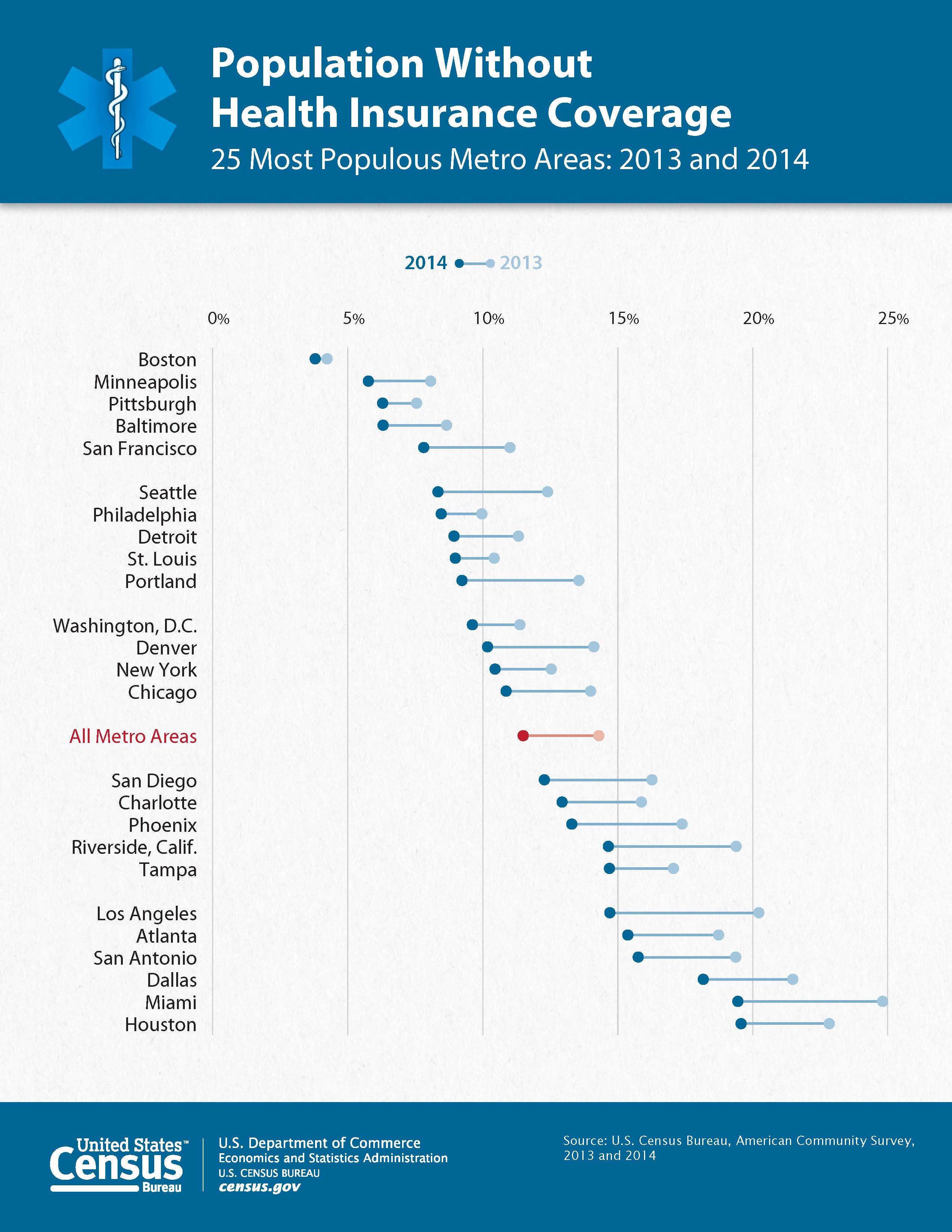
R+ggplot2 version of the "dumbbell" plot at http://census.gov/content/dam/Census/newsroom/releases/2015/cb15-158_graphic_acs_metro.jpg
This hit #rstats today:
Has anyone made a dumbbell dot plot in #rstats, or better yet exported to @plotlygraphs using the API? https://t.co/rWUSpH1rRl
— Ken Davis (@ken_mke) October 23, 2015So, I figured it was worth a cpl mins to reproduce.
While the US gov did give the data behind the chart it was all the data and a pain to work with so I used WebPlotDigitizer to transcribe the points and then some data wrangling in R to clean it up and make it work well with ggplot2.
It is possible to make the top "dumbbell" legend in ggplot2 (but not by using a guide) and color the "All Metro A
hrbrmstr
/ coord_proj.R
Last active
December 27, 2017 13:52
coord_proj - see the rpub : http://rpubs.com/hrbrmstr/coord-proj for examples and this blog post : http://rud.is/b/2015/07/24/a-path-towards-easier-map-projection-machinations-with-ggplot2/ for more 'splainin
This file contains hidden or bidirectional Unicode text that may be interpreted or compiled differently than what appears below. To review, open the file in an editor that reveals hidden Unicode characters.
Learn more about bidirectional Unicode characters
| #' @export | |
| coord_proj <- function(proj="+proj=robin +lon_0=0 +x_0=0 +y_0=0 +ellps=WGS84 +datum=WGS84 +units=m +no_defs", | |
| inverse = FALSE, degrees = TRUE, | |
| ellps.default="sphere", xlim = NULL, ylim = NULL) { | |
| try_require("proj4") | |
| coord( | |
| proj = proj, | |
| inverse = inverse, | |
| ellps.default = ellps.default, | |
| degrees = degrees, |
hrbrmstr
/ README.md
Created
July 11, 2015 14:12
Slight optimizations to http://rpubs.com/walkerke/txlege
Main differences are:
- All the initial data acquisition & munging is kept in one pipeline and the data structure is kept as a
tbl_df - I ended up having to use
html_sessionsince the site was rejecting the access (login req'd) w/o it - The
forloop is now anapplyiteration andpbapplygives you a progress bar for free which is A Good Thing given how long that operation took :-) - The move to
pbapplymakes it possible to do the row-binding and left-joining in a single pipeline, which keeps everything in atbl_df. - Your
forsolution can be made almost as efficient if you do aimg_list <- vector("list", 150)so the list size is pre-allocated.
BTW: the popup code is brilliant and tigris is equally as brilliant!
This file has been truncated, but you can view the full file.
This file contains hidden or bidirectional Unicode text that may be interpreted or compiled differently than what appears below. To review, open the file in an editor that reveals hidden Unicode characters.
Learn more about bidirectional Unicode characters
| { | |
| "cells": [ | |
| { | |
| "cell_type": "code", | |
| "execution_count": 1, | |
| "metadata": { | |
| "collapsed": true | |
| }, | |
| "outputs": [], | |
| "source": [ |
ramhiser
/ leaflet-county-explorer.r
Created
May 4, 2015 18:25
Leaflet app in R to explore U.S. Census demographics by county
This file contains hidden or bidirectional Unicode text that may be interpreted or compiled differently than what appears below. To review, open the file in an editor that reveals hidden Unicode characters.
Learn more about bidirectional Unicode characters
| # TODO: Add a Shiny dropdown to select demographic variable | |
| library(leaflet) | |
| library(noncensus) | |
| library(dplyr) | |
| data("counties", package="noncensus") | |
| data("county_polygons", package="noncensus") | |
| data("quick_facts", package="noncensus") | |
| counties <- counties %>% |
NewerOlder